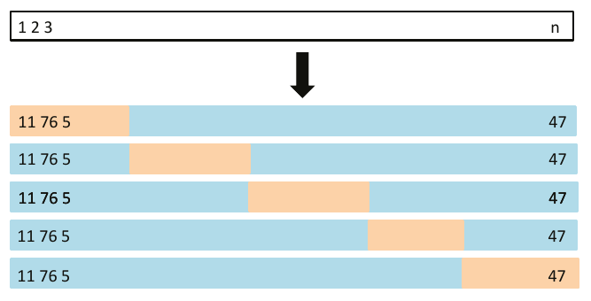
# Function to
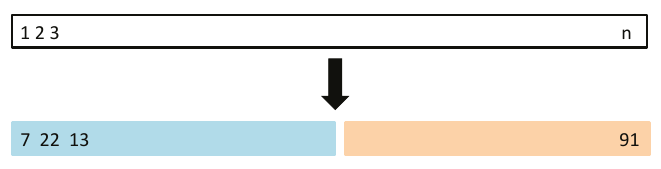
# 1. split the data proportionaly into training and evaluation sample,
# 2. fit the linear model given by formula to training set,
# 3. calculate MSE based on evaluation set.
# in: formula - formula defining relationship among variables,
# data - data frame to split
# proportion - numeric value in [0,1] interval, proportion of training sample to the whole set
# out: numeric value of MSE
mse_validset_lm <- function(formula, data, proportion = 1/2, seed = sample(1000,1)) {
n <- nrow(data)
set.seed(seed)
ind <- 1:n %in% sample(n, size = n*proportion)
train <- data[ind,]
valid <- data[!ind,]
fit <- lm(formula, train)
yname <- names(fit$model)[[1]]
RSS <- sum((valid[[yname]] - predict(fit, newdata = valid))^2)
df <- nrow(valid) - length(fit$coefficients)
RSS / df
}
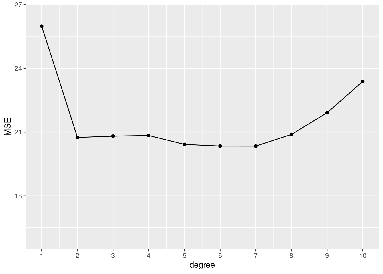
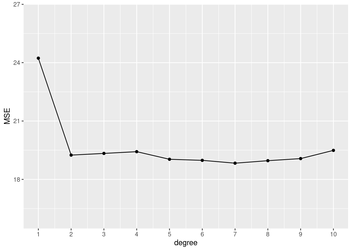
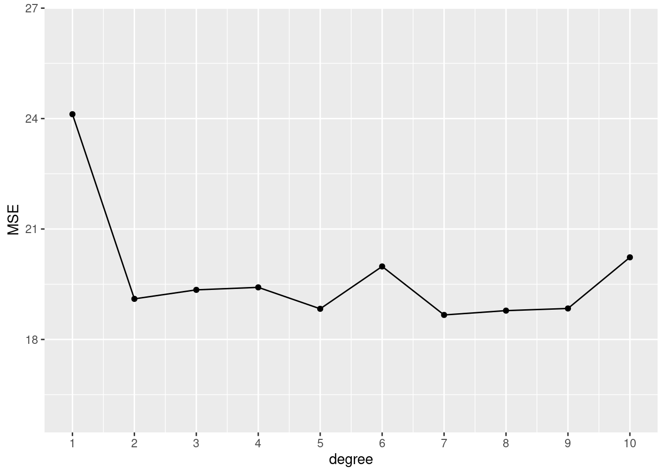
# 1 split, 10 polynomials of certain degrees
tibble::tibble(
degree = 1:10,
MSE = sapply(degree, function(x) mse_validset_lm(mpg ~ poly(horsepower, x),
ISLR2::Auto,
seed = 2))
) |>
ggplot() + aes(x = degree, y = MSE) +
geom_line() + geom_point() +
scale_x_continuous(n.breaks = 10) +
ylim(16, 26.5)
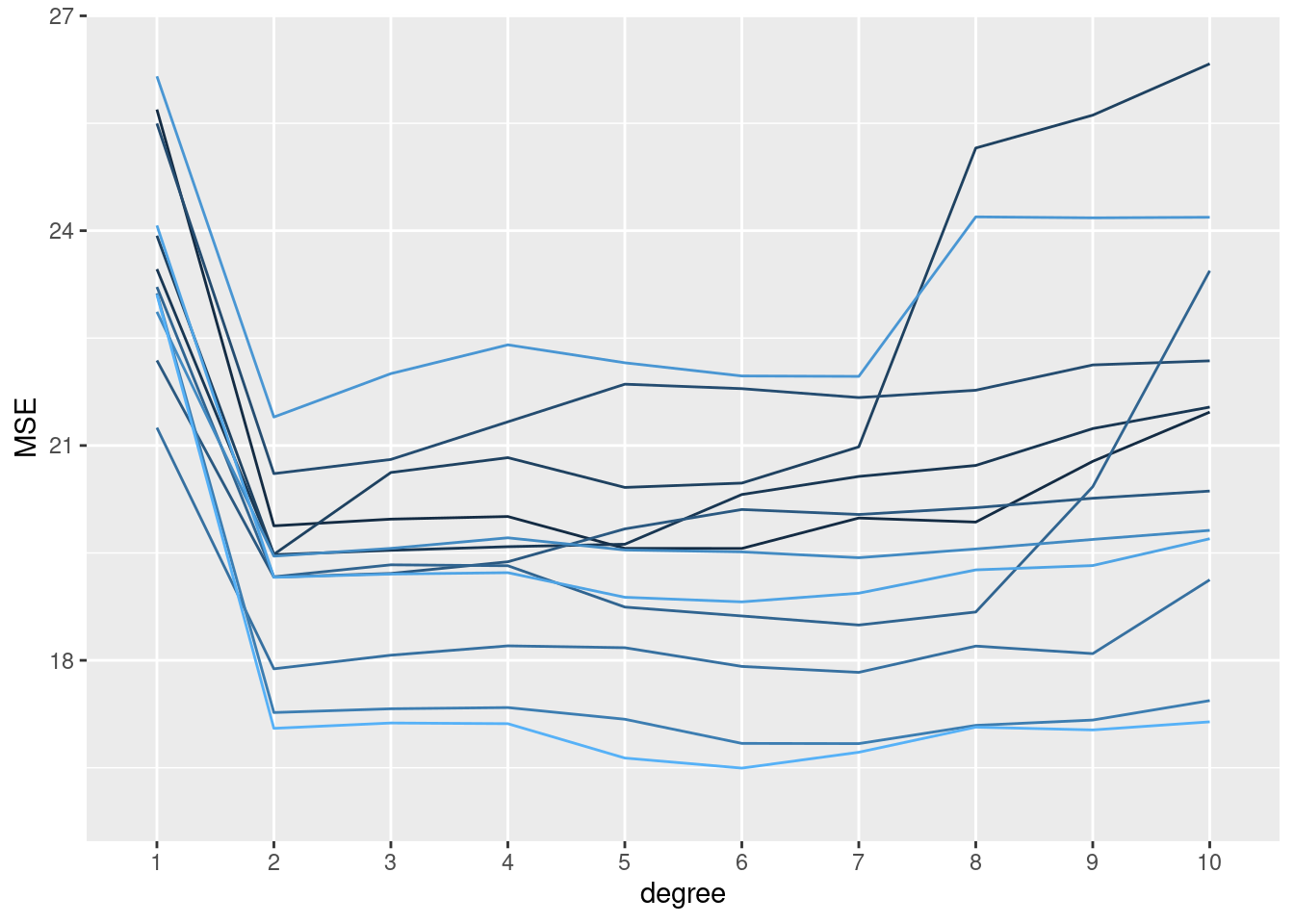
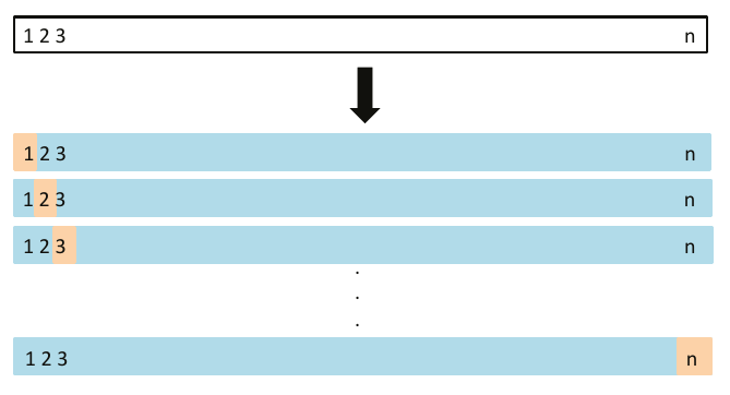
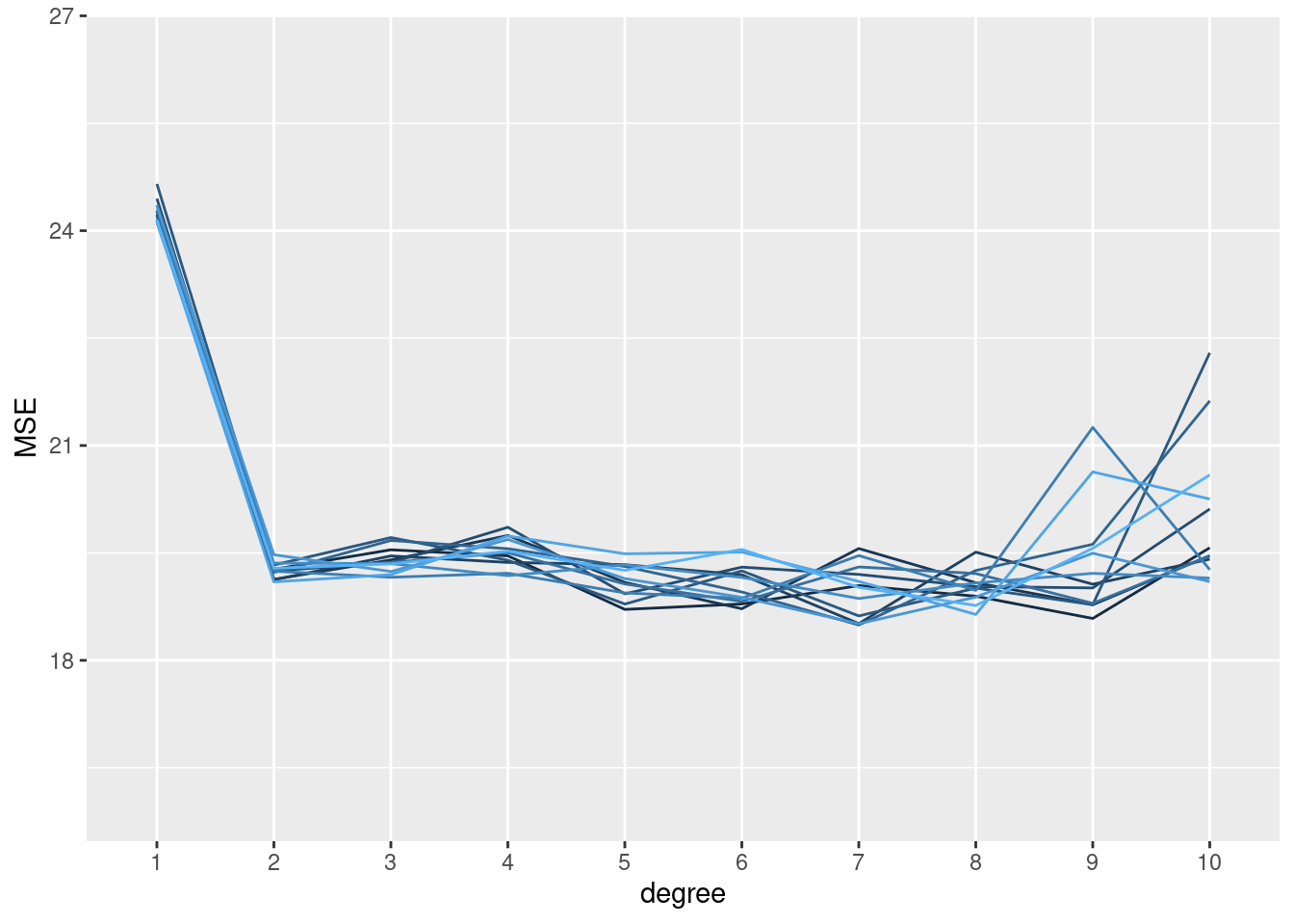
# 12 splits, 10 models
set.seed(1234)
replicate(n = 12, local({
seed <- sample(1000, 1)
sapply(1:10, function(x) mse_validset_lm(mpg ~ poly(horsepower, x),
ISLR2::Auto, seed = seed))
})
) |>
t() |> as.data.frame() |>
setNames(1:10) |>
dplyr::mutate(replication = 1:dplyr::n()) |>
tidyr::pivot_longer(-replication, names_to = "degree", values_to = "MSE",
names_transform = forcats::as_factor) |>
ggplot() + aes(x = degree, y = MSE, color = replication, group = replication) +
geom_line(show.legend = FALSE) +
ylim(16, 26.5)