4 Statistical modelling
All of the methods already discussed are either a model itself, part of a model or method based on a model – from mean value through simple tests to whole probability distribution.
A statistical model is a mathematical model that embodies a set of statistical assumptions concerning the generation of sample data. (Wikipedia)
Its purpose is to help
- understand the mechanism behind sample (inference about the whole population),
- generate new data (predict, “what if”).
Statistical model specifies mathematical relationships between one or more RVs, so the type of RV (again) strongly determines a set of appropriate models.
The most complex models can provide joint probability distribution of all RVs involved, however we restrict ourselves here to the most commonly used class
- that aims to describe distribution of one dependent RV called response
- with the help of independent (possibly random) variables called predictors (or covariates, features, explanatory variables).
This class of models is often refered to as supervised statistical learning or predictive statistical models. According to the type of response, they solve
- either regression task (when response is continuous),
- or classification task (for categorical response).
Code
# load additional packages
library(ggplot2)

# elementary transformations before analysis is applied
dat <- mtcars |>
  dplyr::transmute(
    mileage = mpg,
    cylinders = as.factor(cyl),
    horsepower = hp,
    displacement = disp,
    weight = wt,
    transmission = dplyr::recode(am, `0` = "automatic", `1` = "manual")
    )
n <- nrow(dat)
4.1 Continuous response
In the general additive case, a stochastic model with continuous response consists of a sum of predictable (deterministic) and unpredictable (stochastic) part, i.e. \[ Y = E(Y|\vec{X}) + \varepsilon \] where \(\vec{X}=\{X_1,\ldots,X_p\}\) stands for predictors and the residual term \(\varepsilon\) represents noise with a given distribution. Thus the model of response variable distribution is split into mean value and the remainder.
4.1.1 Linearity in parameters
The conditional mean \(E(Y|\vec{X})\) represents a regression function that does not need to be linear in predictors but that is usually chosen to be a linear function of parameters, i.e. \[ \begin{split} E(Y|\vec{X}) &= b_1f_1(\vec{X}) + \ldots + b_mf_m(\vec{X}) \\ &= (b_1,\ldots,b_m)\cdot\Big(f_1(\vec{X}),\dots,f_m(\vec{X})\Big) \end{split} \] where \(b_j\) are parameters and \(f_j:R^p\to R\) are basis functions. As a convention, \(f_1\equiv1\), then \(b_1\) is called intercept.
Given a sample \(\{y_i,\vec{x}_i\} = \{y_{i},x_{i1},\ldots,x_{ip}\}_{i=1}^n\), models linear in parameters are easily estimable by method of least squares. Let us write the statistical model as system of observation equations, \[ \begin{split} y_i &= \Big(f_1(\vec{x}_i),\ldots,f_m(\vec{x}_i)\Big)\cdot\mathbf{b} + \varepsilon_i, \qquad\text{for}\quad i=1,\ldots,n,\\ \text{that is}\qquad\mathbf{y} &= \mathbf{X} \mathbf{b} + \boldsymbol{\varepsilon}, \end{split} \] where \(\mathbf{X}\) is the so-called design matrix (or regression/model matrix) of dimension \(n\times m\), \(\mathbf{b}\) is vector of parameters, \(\mathbf{y}\) response values and \(\boldsymbol{\varepsilon}\) residuals.
Least squares estimates of \(\mathbf{b}\) are those that minimize residuals sum of squares \(\boldsymbol{\varepsilon}'\boldsymbol{\varepsilon}\), which is obviously a function of parameters through equation \(\boldsymbol{\varepsilon} = \mathbf{y} - \mathbf{X} \mathbf{b}\). To find extreme of a smooth function, one needs to find point where derivative is zero. \[ \begin{split} \frac{\partial\ (\mathbf{y} - \mathbf{X} \mathbf{b})'(\mathbf{y} - \mathbf{X} \mathbf{b})}{\partial\mathbf{b}} = -2\mathbf{X}'(\mathbf{y} - \mathbf{X} \mathbf{b}) & \\ \mathbf{X}'\mathbf{y} - \mathbf{X}'\mathbf{X} \hat{\mathbf{b}} &= \mathbf{0} \\ \mathbf{X}'\mathbf{X} \hat{\mathbf{b}} &= \mathbf{X}'\mathbf{y} \\ \hat{\mathbf{b}} &= (\mathbf{X}'\mathbf{X})^{-1}\mathbf{X}'\mathbf{y} \end{split} \] Then estimates of response, residue and residual variance are, respectively, given by \[ \begin{split} E(Y|\mathbf{X}) \equiv \hat{\mathbf{y}} &= \mathbf{X} \hat{\mathbf{b}}, \\ \hat{\boldsymbol{\varepsilon}} &= \mathbf{y} - \hat{\mathbf{y}},\\ \hat\sigma_{\varepsilon}^2 &= \frac{\hat{\boldsymbol{\varepsilon}}'\hat{\boldsymbol{\varepsilon}}}{n-m} \end{split} \] and the covariance matrix of parameters estimate is calculated from formula \[ \hat{\boldsymbol{\Sigma}}_b=\hat\sigma_{\varepsilon}^2(\mathbf{X}'\mathbf{X})^{-1}. \] Variances \(\sigma_{b_j}^2\) located on diagonal of \(\boldsymbol{\Sigma}_b\) serves for testing significance of parameters \(b_j\) through the test statistic \[ \frac{\hat b_j}{\hat\sigma_{b_j}}\sim t(n-m) \] which is valid only if the model assumptions hold.
Linear model assumes that
- the relationship of response with predictors via basis functions is formulated correctly,
- residuals are
- uncorrelated and normally distributed, no outliers,
- with constant variance (homoscedasticity),
- uncorrelated with predictors,
- there is little or no multicollinearity among (basis functions of) predictors.
4.1.2 One continuous predictor
The simplest model of two variables assumes linear relationship between them, \[ Y = b_1 + b_2 X + \varepsilon \] where parameters \(b_1,b_2\) are called intercept and slope, respectively.
Let us build a linear regression model of mileage explained by weight. Scatter plot of the two RVs unveils roughly linear relationship, so the linearity assumption of the model could be satisfied.
Code
dat |>
  ggplot() + aes(x = weight, y = mileage) +
  geom_point() +
  stat_smooth(geom = "line", method = "lm", formula = y ~ x, color = 4)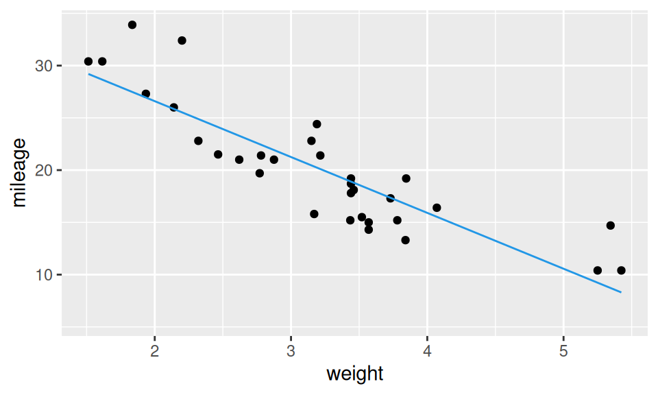
Code
fit1 <- lm(mileage ~ weight, dat)
fit1 |> summary() |> pander::pander(caption="")| Estimate | Std. Error | t value | Pr(>|t|) | |
|---|---|---|---|---|
| (Intercept) | 37.29 | 1.878 | 19.86 | 8.242e-19 |
| weight | -5.344 | 0.5591 | -9.559 | 1.294e-10 |
| Observations | Residual Std. Error | \(R^2\) | Adjusted \(R^2\) |
|---|---|---|---|
| 32 | 3.046 | 0.7528 | 0.7446 |
The first table of the estimated model is dedicated to parameter estimates, the second one summarizes the model as a whole. Few comments are necessary here:
- The value of intercept means intersection of the regression line with y-axis, however in this case it has no practical meaning, since there are no cars with zero weight.
- Slope parameter is labeled by the associated RV (here the basis function is the so-called “identity”) and represent a change in mileage when weight is increased by 1 (i.e., 1000 pounds).
- Standard errors help to evaluate precision of parameters estimate and their distinguishability from zero. Here t value (test statistic = estimate / std.error) is out of the 95% probability interval of t-distribution, which is roughly (-2,2), thus the effect of weight is significant. The same information is conveyed by p-value not exceeding 5%.
- Coefficient of determination \(R^2\) is a very basic goodness-of-fit measure ranging from 0 (useless model) to 1 (perfect fit). It is defined as \[ R^2=1-\frac{\sum_i\hat\varepsilon_i^2}{\sum_i(y_i-m_Y)^2} \] In this case of single predictor it coincides with squared Pearson correlation coefficient. One drawback of \(R^2\) is that it increases with number of predictors (whatever effect they have), that’s why the adjusted version is usually also reported, given by formula \(adjR^2=1-\hat\sigma_\varepsilon^2/\hat\sigma_Y^2 = 1-(1-R^2)\frac{n-1}{n-m}\).
A series of diagnostic plots (mainly on residuals) can be used to evaluate model.
Code
ggfortify:::autoplot.lm(fit1)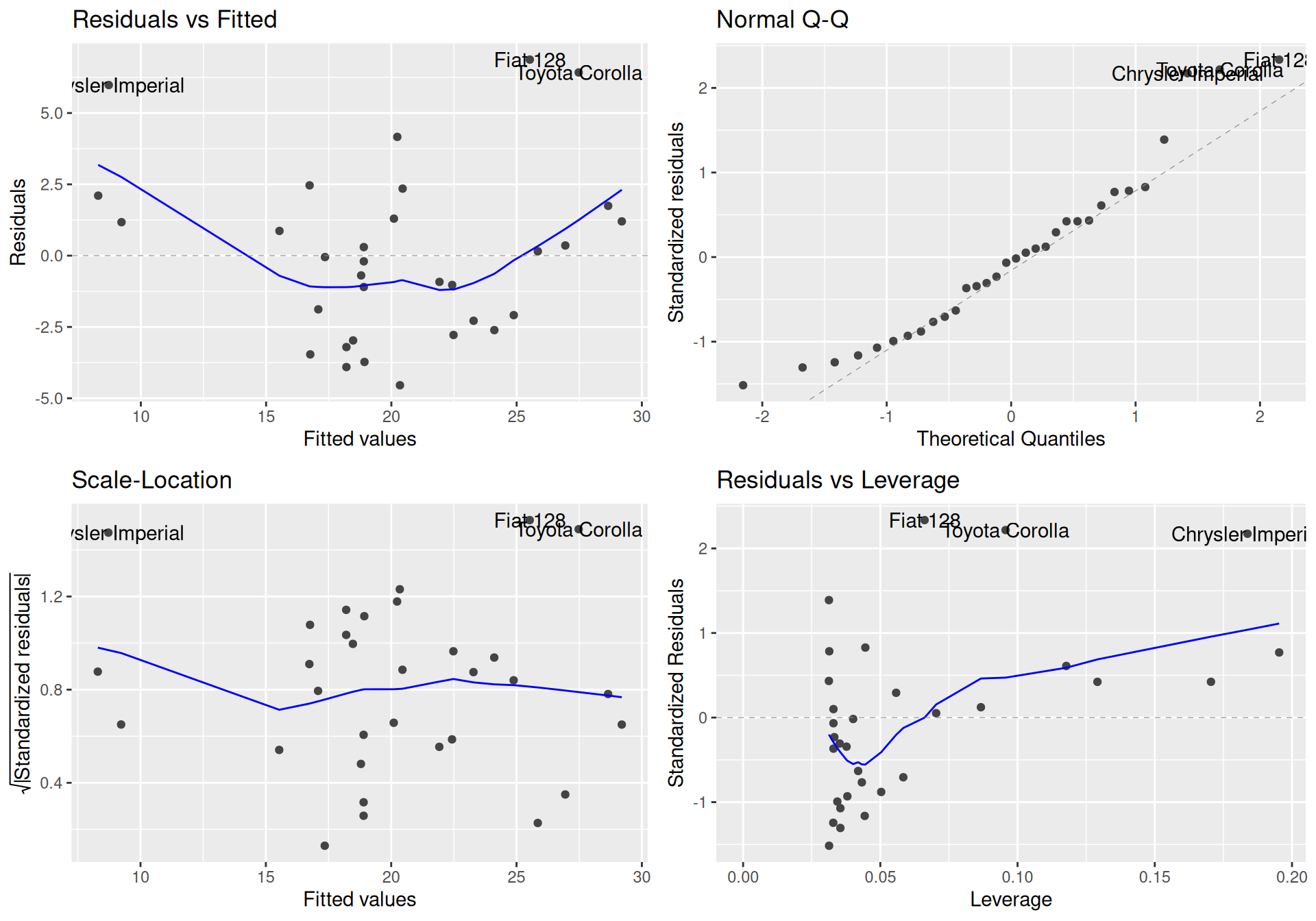
Residuals should be concentrated evenly around horizontal zero line in the left plots (homoscedasticity and linearity assumptions), as well as around identity line in quantile-quantile plot (normality assumption). The last plot quantifies leverage effect of individual observations on the model. In this particular case we see extraordinarity of three cars, which may be responsible for slightly curvilinear shape of the points cloud.
As a nonlinear alternative let us try parabolic fitting curve by adding a quadratic term (power basis function). \[ Y = b_1 + b_2 X + b_3 X^2+ \varepsilon \]
Code
fit2 <- lm(mileage ~ weight + I(weight^2), dat)
dat |>
ggplot() + aes(x = weight, y = mileage) +
geom_point() +
stat_smooth(geom = "line", method = "lm", formula = y ~ x + I(x^2), color = 4)
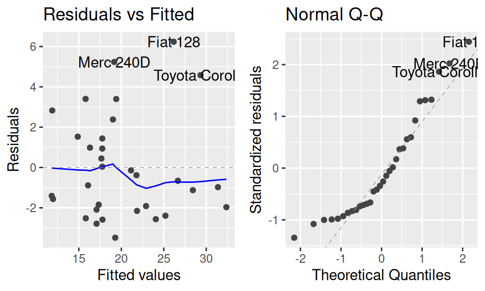
ggfortify:::autoplot.lm(fit2, which = 1:2)
fit2 |> summary() |> pander::pander(caption="")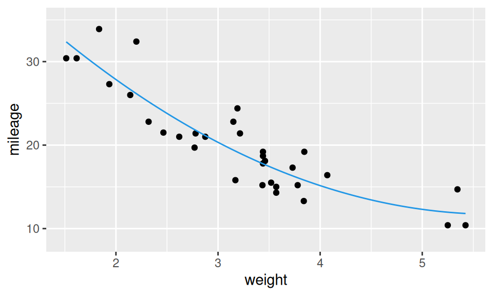
| Estimate | Std. Error | t value | Pr(>|t|) | |
|---|---|---|---|---|
| (Intercept) | 49.93 | 4.211 | 11.86 | 1.213e-12 |
| weight | -13.38 | 2.514 | -5.322 | 1.036e-05 |
| I(weight^2) | 1.171 | 0.3594 | 3.258 | 0.00286 |
| Observations | Residual Std. Error | \(R^2\) | Adjusted \(R^2\) |
|---|---|---|---|
| 32 | 2.651 | 0.8191 | 0.8066 |
Naturally, the extended model fits the data better. But (!) is the gain worth the higher complexity (lower interpretability)? This question can be answered from several perspectives. For instance, by
- testing significance of additional (in-sample) variance explained,
- comparing (out-of-sample) mean prediction error, e.g. by cross-validation.
The first approach employs ANOVA test comparing two nested models.
Code
anova(fit1, fit2) |> pander::pander(missing="")| Res.Df | RSS | Df | Sum of Sq | F | Pr(>F) |
|---|---|---|---|---|---|
| 30 | 278.3 | ||||
| 29 | 203.7 | 1 | 74.58 | 10.61 | 0.00286 |
The second approach requires repeating of the following procedure 1. split data into two samples – train and test, 2. fit models to train sample, 3. make predictions for points in test sample and calculate prediction error and aggregation (usually by averaging) of prediction errors from all runs into single value.
Code
# cross validation
set.seed(1)  # for reproducibility
mse_cv_lm <- function(lmfits, data, nfolds) {
  # preliminary
  formulas <- sapply(lmfits, as.formula)
  variables_name <- lapply(formulas, function(x) all.vars(x))
  response_name <- variables_name |> sapply(function(x) x[1]) |> unique()
  # error handling
  stopifnot(all(unique(unlist(variables_name) %in% names(data))),
            length(response_name) == 1
            )
  # calculation
  sapply(
    split(1:nrow(dat), f = sample(rep(1:nfolds, length.out = nrow(data)))), # row indices
    function(ind) {  # MSE in each fold
      formulas |>
        lapply(function(x) predict(lm(x, data[-ind,]), newdata = data[ind,])) |>
        sapply(function(x) sum((data[ind, response_name] - x)^2))
    }) |>
    rowMeans()
}

list(linear = fit1, quadratic = fit2) |>
  mse_cv_lm(dat, 5) |>
  round(1) |> rbind("CV MSE" = _)
linear quadratic
CV MSE 65 51.4From both methods the quadratic model comes out as more appropriate.
4.1.3 One discrete predictor
As before, we need to distinguish between nominal, ordinal and other discrete random variables.
Ordinal RVs can be treated as continuous only if “distances” between categories (levels) can be considered as approximately equal (like counts, or questionnaire answers in Likert scale). On the other hand, non-equidistant ordinal and nominal RVs need to be recoded to the so-called dummy (or indicator) variables.
“Dummies” are binary variables indicating occurrence of specific value of the original RV. Their number is one less than cardinality of the RV to be recoded, just to prevent redundancy (and thus collinearity, see later). The omitted level is treated as reference level and its choice is important only from the viewpoint of parameters interpretation.
Since dummy coding of dichotomous RV is trivial (values are directly mapped to \(\{0,1\}\) set), let us illustrate the matter on number of cylinders. Suppose the difference between 4 and 6 cylinder engines is distinct from difference between those with 6 and 8 cylinders. We create dummy variables \(\mathbf{1}_{\{6\}}(X)\) and \(\mathbf{1}_{\{8\}}(X)\), defined with indicator function \[ \mathbf{1}_{A}(x) = \begin{cases}1 & \text{for }x\in A\\0 & \text{otherwise}\end{cases} \] so that the stochastic model of mileage \(Y\) and number of cylinders \(X\) can be written as \[ \begin{split} Y &= b_1 + b_2\mathbf{1}_{\{6\}}(X) + b_3\mathbf{1}_{\{8\}}(X) + \varepsilon\\ &= \begin{cases} b_1 & \text{if}\ X = 4 \\ b_1 + b_2 & \text{if}\ X = 6 \\ b_1 + b_3 & \text{if}\ X = 8 \end{cases} \quad +\varepsilon \end{split} \] and the corresponding design matrix has three columns. The model can be visualized as three points.
Code
fit <- lm(mileage ~ cylinders, dat)
means <- levels(dat$cylinders) |> as.factor() |>
  data.frame(cylinders = _) |>
  (\(x) cbind(x, mileage = predict(fit, newdata = x)))()
dat |>
  ggplot() + aes(x = cylinders, y = mileage) +
  geom_point() +
  geom_point(data = means, color = 4, size = 3) +
  geom_line(aes(group = 1), data = means, color = 4, linetype = 2)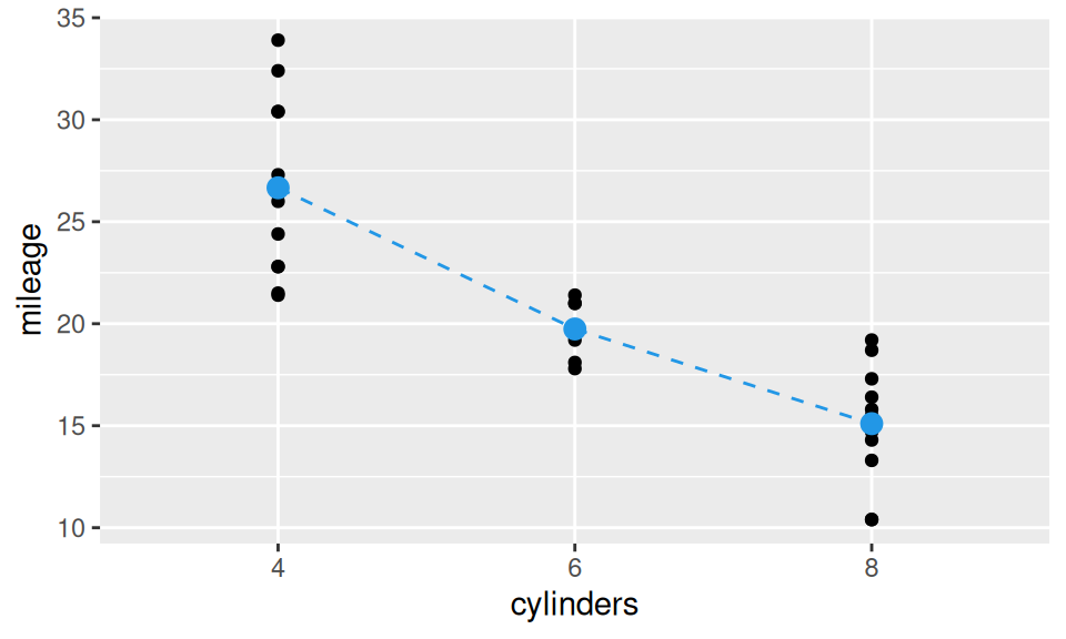
4.1.4 Multiple predictors
With more than one predictor we should
- be aware of possible existence of interactions among them,
- be concerned by multicollinearity,
- select only valuable predictors from among all features available.
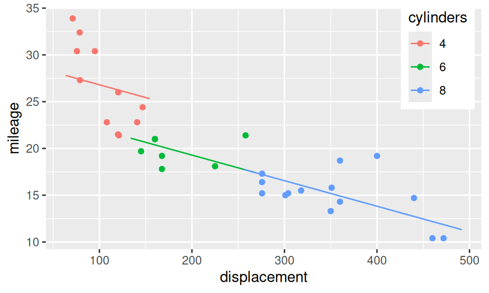
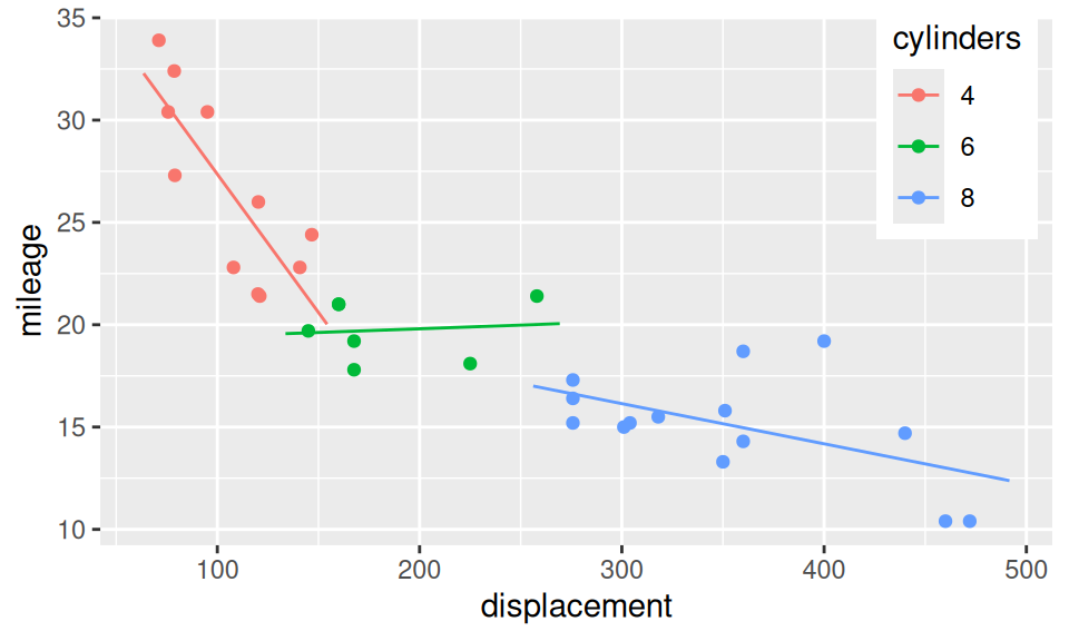
Interaction is a joint effect of two (or more) predictors on response, in the sense that, effect of one predictor is different for (e.g.) smaller values of another predictor than for larger values. Let us build three regression models of mileage (\(Y\)): the first one has only displacement (\(X_1\)) as explanatory variable, the second adds number of cylinders (\(X_2\)) and the third considers also their multiplication. \[ \begin{split} (M1)\qquad Y &= b_1 + b_2X_1 + \varepsilon \\ (M2)\qquad Y &= b_1 + b_2X_1 + b_3\mathbf{1}_{\{6\}}(X_2) + b_4\mathbf{1}_{\{8\}}(X_2) + \varepsilon \\ (M3) \qquad Y &= b_1 + b_2X_1 + b_3\mathbf{1}_{\{6\}}(X_2) + b_4\mathbf{1}_{\{8\}}(X_2) + b_5X_1 \mathbf{1}_{\{6\}}(X_2) + b_6X_1 \mathbf{1}_{\{8\}}(X_2)\\ &= \begin{cases} b_1 + b_2X_1 & \text{if}\ X_2=4\\ (b_1 + b_3) + (b_2 + b_5)X_1 & \text{if}\ X_2=6 \\ (b_1 + b_4) + (b_2 + b_6)X_1 & \text{if}\ X_2=8 \\ \end{cases}\quad + \varepsilon \end{split} \]
Code
# grid of predictors (two end points for displacement are enough)
xgrid <- dat |>
  dplyr::reframe(displacement = modelr::seq_range(displacement, n = 2, expand = 0.2),
                 .by = cylinders) |>
  dplyr::arrange(cylinders)

# fitting models
fit1 <- lm(mileage ~ displacement, dat)
fit2 <- lm(mileage ~ displacement + cylinders, dat)
fit3 <- lm(mileage ~ displacement * cylinders , dat)

# plots
g <- ggplot(dat) + aes(x = displacement, y = mileage) +
  geom_point() +
  theme(legend.position = "inside", legend.position.inside = c(0.9, 0.8))

g + geom_line(data = xgrid |> modelr::add_predictions(fit1, var = "mileage"))
g + aes(color = cylinders) +
  geom_line(data = xgrid |> modelr::add_predictions(fit2, var = "mileage"))
g + aes(color = cylinders) +
  geom_line(data = xgrid |> modelr::add_predictions(fit3, var = "mileage"))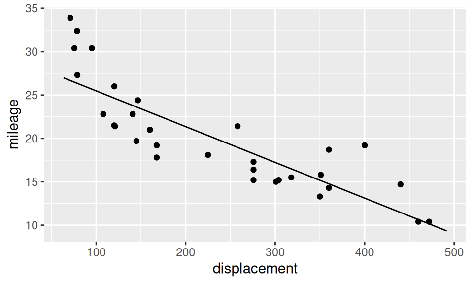
Code
# model summary
fit1 |> pander::pander(caption = "")
fit2 |> pander::pander(caption = "")
fit3 |> pander::pander(caption = "")| Estimate | Std. Error | t value | Pr(>|t|) | |
|---|---|---|---|---|
| (Intercept) | 29.6 | 1.23 | 24.07 | 3.577e-21 |
| displacement | -0.04122 | 0.004712 | -8.747 | 9.38e-10 |
| Estimate | Std. Error | t value | Pr(>|t|) | |
|---|---|---|---|---|
| (Intercept) | 29.53 | 1.427 | 20.7 | 1.637e-18 |
| displacement | -0.02731 | 0.01061 | -2.574 | 0.01564 |
| cylinders6 | -4.786 | 1.65 | -2.901 | 0.007169 |
| cylinders8 | -4.792 | 2.887 | -1.66 | 0.1081 |
| Estimate | Std. Error | t value | Pr(>|t|) | |
|---|---|---|---|---|
| (Intercept) | 40.87 | 3.02 | 13.53 | 2.791e-13 |
| displacement | -0.1351 | 0.02791 | -4.842 | 5.096e-05 |
| cylinders6 | -21.79 | 5.307 | -4.106 | 0.0003542 |
| cylinders8 | -18.84 | 4.612 | -4.085 | 0.0003743 |
| displacement:cylinders6 | 0.1387 | 0.03635 | 3.817 | 0.0007528 |
| displacement:cylinders8 | 0.1155 | 0.02955 | 3.909 | 0.0005923 |
Clearly, interactions play a big role here, since the effect of displacement on mileage varies across cylinders. The third model also shows, that cars with small number of cylinders are inefficient with large displacement and vice-versa. However, the seemingly positive slope for 6 cylinder engines is a nonsense, and from an experience the green line should bridge the other two lines. There are too few cars with 6 cylinders to get significant slope for the middle segment (\(b_2+b_5 \ll SE_{b_2+b_5}\)). A more reliable model would be obtained from extended dataset.
According to ANOVA test, inclusion of cylinders improved the fit significantly, and even more with the interactions.
Code
anova(fit1, fit2, fit3) |> pander::pander(missing="", caption="")| Res.Df | RSS | Df | Sum of Sq | F | Pr(>F) |
|---|---|---|---|---|---|
| 30 | 317.2 | ||||
| 28 | 243.6 | 2 | 73.54 | 6.537 | 0.005012 |
| 26 | 146.2 | 2 | 97.39 | 8.657 | 0.001313 |
Multicolinearity is a phenomenon, when one or several predictors are linear combination of the others. As a consequence the inference about model parameters suffers a lot, because with higher standard errors even strong effects may appear insignificant.
To detect multicollinearity, one may check correlations among predictors or calculate the so-called variation inflation factor \(VIF=\frac{1}{1-R_j^2}\) where \(R_j^2\) is associated with regression of j-th predictor on the other predictors. VIF reaches minimum in 1 (no colinearity) and above 5 it announces trouble.
The remedy to multicolinearity is either in manual eliminating all redundant predictors, or applying some automatic procedure for feature selection, e.g., step-wise selection and regularization, or for dimensionality reduction such as principal component analysis.
4.2 Discrete response
Modelling distribution of discrete random variables by regression is a bit trickier than modelling the continuous one. And again, we need to distinguish between binary (dichotomous), nominal and ordinal case. Neglecting the discrete nature of RVs domain and treating them as continuous (in order to use ordinary regression) means forcing
- binary RV to have hardly interpretable model, moreover
- ordinal RV to get redefined distance between values, and moreover
- nominal RV to have ordered values.
In data mining and machine learning terminology the problem of predicting discrete response is called classification task (as opposed to regression task for continuous response).
Philosophically, there are two groups of methods for probabilistic classification:
- discriminative, where conditional probability for response is modelled directly,
- generative, that fits the joint distribution of predictors and use Bayes theorem to get conditional probability for response.
4.2.1 Binary
Binary RV needs to be recoded to \(\{0,1\}\) domain so that occurence of one its value (class) is treated in terms of probability as function of some predictors \(\vec X = (X_1,\ldots,X_p)\), \[
p(\vec X)\equiv Pr(Y=1|\vec X).
\]
Approximating \(p(\vec X)\) by linear function of \(\vec X\) is not satisfactory, because probability cannot exceed \([0,1]\) interval. However, by applying appropriate transformation, e.g., logistic function \(h(x) = (f_2\circ f_1)(x) = \frac{e^x}{1+e^{x}}\), where
- exponential function \(f_1(x)=e^x\) makes 0 to be the lower bound,
- hyperbolic function \(f_2=\frac{x}{1+x}\) restricts the outcome to 1 from above,
we may link the probability to (the so called) linear predictor \((b_1,\ldots b_p)\cdot(X_1,\ldots X_p)\), so that in case of single feature \(X\) the formula is given by \[
\begin{split}
\text{(probability)} \qquad
p(X) &= \frac{e^{b_1+b_2X}}{1+e^{b_1+b_2X}} \\
\text{(odds ratio)}\qquad
\frac{p(X)}{1-p(X)} &= e^{b_1+b_2X} \\
\text{(log odds)} \qquad
\ln\left(\frac{p(X)}{1-p(X)}\right) &= b_1+b_2X.
\end{split}
\] This is a fundament of the so called logistic regression. Its parameters are well interpretable:
- similarly to linear regression, monotonicity depends on the sign of parameter \(b_2\),
- increasing \(X\) by 1 changes the odds ratio \(e^{b_2}\)-times,
- higher the \(|b_2|\), steeper the transition between 0 and 1,
- \(p\left(-\frac{b_1}{b_2}\right)=\frac12\), which is the usual classification threshold.
Parameters are estimated by maximizing logarithm of likelihood function \[ \begin{split} L(b_1,b_2) &= \prod_{i=1}^n Pr(Y=y_i|X=x_i) \\ &= \prod_{i=1}^n p(x_i)^{y_i}\big(1-p(x_i)\big)^{1-y_i} \end{split} \] that incorporates density of Bernoulli distribution. Due to variable dispersion, solution to this optimisation problem needs to be found iteratively via Newton method.
Let us illustrate logistic regression on the relation between gear transition type and car weight.
Code
obs <- dat |>
dplyr::mutate(manual = dplyr::case_match(transmission,
"automatic" ~ 0,
"manual" ~ 1)
)
fitLin <- lm(manual ~ weight, data = obs)
predLin <- data.frame(
weight = modelr::seq_range(dat$weight, n = 2, expand = 0.2)
) |>
modelr::add_predictions(model = fitLin, "manual")
ggplot() + aes(x = weight, y = manual) +
geom_point(data = obs) +
geom_line(data = predLin, color = 2)
fitLog <- glm(manual ~ weight, family = "binomial", data = obs)
predLog <- data.frame(
weight = modelr::seq_range(dat$weight, n = 30, expand = 0.2)
) |>
modelr::add_predictions(model = fitLog, "manual", type = "response")
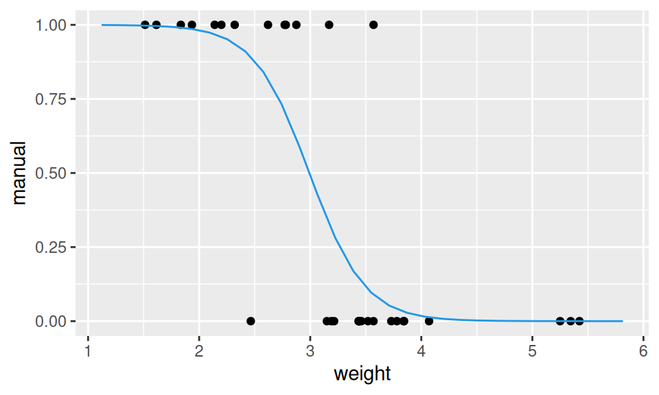
ggplot() + aes(x = weight, y = manual) +
geom_point(data = obs) +
geom_line(data = predLog, color = 4)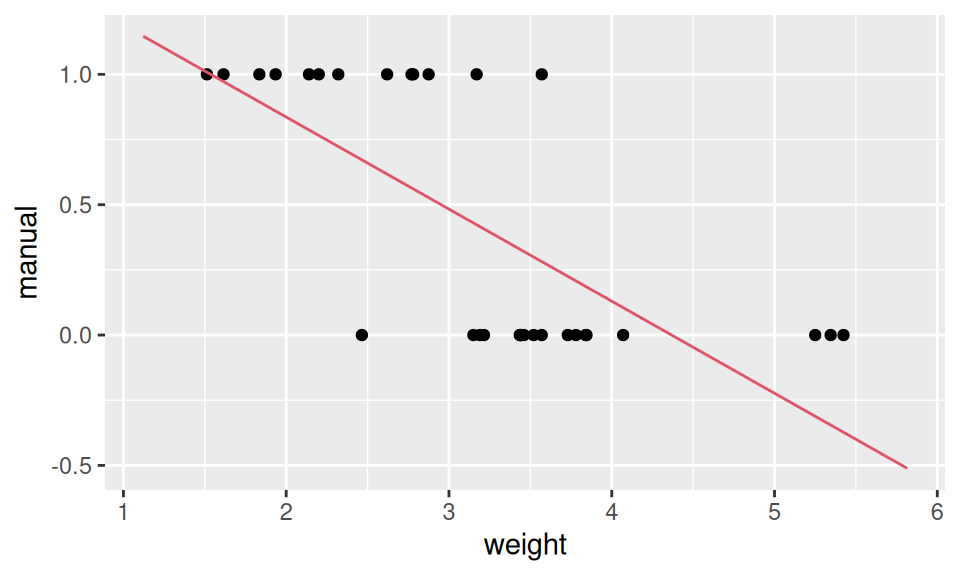
Code
fitLog |> summary() |> pander::pander()| Estimate | Std. Error | z value | Pr(>|z|) | |
|---|---|---|---|---|
| (Intercept) | 12.04 | 4.51 | 2.67 | 0.007588 |
| weight | -4.024 | 1.436 | -2.801 | 0.005088 |
(Dispersion parameter for binomial family taken to be 1 )
| Null deviance: | 43.23 on 31 degrees of freedom |
| Residual deviance: | 19.18 on 30 degrees of freedom |
From the output we see negative dependence between weight and (manual) transmission, and the decision boundary at \(X = -\frac{12}{-4}=3\).
Comparing to linear regression, the output of logistic regression (as a subclass of Generalized linear models) contains a new measure – deviance – instead of variance.
- Residual deviance \(D\) is defined as difference between log-likelihood functions of a saturated (i.e. perfect fitting) and our model. Since likelihood of perfect model is equal to 1, its logarithm to 0, then residual deviance \(D=-2\ln L(\hat b_1, \hat b_2)\) is always non-negative.
- Null deviance is a reference value corresponding to constant model (with no predictors), \(D_0=-2\ln L(\hat b_1|b_2=0)\).
- Multiplying by 2 ensures that its asymptotic distribution is \(\chi^2\).
- Sometimes also Akaike (or some other) information criterion is reported, defined as \(AIC=D+2k\), where \(k\) is number of parameters. Information criteria are used to distinguish among models by penalizing complexity. Model with smaller AIC is preferred.
The dependence between transmission and weight seems to be well described by the S-shaped curve, also called first-order logistic curve. In other cases the second-order logistic curve given by the model \[ \ln\left(\frac{p(X)}{1-p(X)}\right) = b_1 + b_2 X + b_3 X^2 \] may be more appropriate.
Code
fitLog2 <- glm(manual ~ horsepower + I(horsepower^2), family = "binomial", data = obs)
predLog2 <- data.frame(
  horsepower = modelr::seq_range(dat$horsepower, n = 30, expand = 0.2)
) |>
  modelr::add_predictions(model = fitLog2, "manual", type = "response")

ggplot() + aes(x = horsepower, y = manual) +
  geom_point(data = obs) +
  geom_line(data = predLog2, color = 4)
fitLog2 |> summary() |> coefficients() |> pander::pander()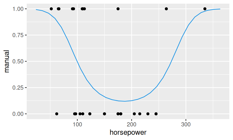
| Estimate | Std. Error | z value | Pr(>|z|) | |
|---|---|---|---|---|
| (Intercept) | 7.166 | 3.119 | 2.297 | 0.02161 |
| horsepower | -0.09828 | 0.04238 | -2.319 | 0.02039 |
| I(horsepower^2) | 0.0002636 | 0.0001265 | 2.084 | 0.03719 |
4.2.2 Nominal
Logistic regression can be generalized to a response with more than two values. One of the values is chosen as a reference class. If it is the last one, say \(K\), then for \(k=1,2,\ldots,K-1\) we get probabilities \[ \begin{split} Pr[Y=k|X=x] &= \frac{e^{b_{k1} + b_{k2}x}}{1 + \sum_{l=1}^{K-1}e^{b_{l1} + b_{l2}x}}, \\ Pr[Y=K|X=x] &= \frac{1}{1 + \sum_{l=1}^{K-1}e^{b_{l1} + b_{l2}x}}, \qquad \text{thus}\\ \log\left(\frac{Pr[Y=k|X=x]}{Pr[Y=K|X=x]}\right) &= b_{k1} + b_{k2}x \end{split} \] An alternative formulation (without setting a reference class) is called softmax, \[ \begin{split} Pr[Y=k|X=x] &= \frac{e^{b_{k1} + b_{k2}x}}{ \sum_{l=1}^{K}e^{b_{l1} + b_{l2}x}} \qquad \text{for}\quad k\in\{1,\ldots, K\} \\ \log\left(\frac{Pr[Y=k_1|X=x]}{Pr[Y=k_2|X=x]}\right) &= (b_{k_11}-b_{k_21}) + (b_{k_12}-b_{k_22})x \qquad \text{for}\quad k_1,k_2\in\{1,\ldots, K\} \end{split} \]
Because there is no nominal variable present in mtcars data, we illustrate the method on the well-known iris dataset.
Code
iris |>
  ggplot() + aes(x = Petal.Width, y = Species) + geom_boxplot()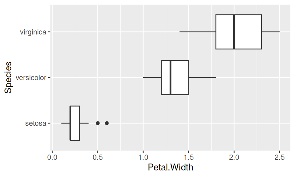
Code
fit <- nnet::multinom(Species ~ Petal.Width, data = iris, trace = FALSE)
fit
Call:
nnet::multinom(formula = Species ~ Petal.Width, data = iris,
trace = FALSE)
Coefficients:
(Intercept) Petal.Width
versicolor -24.08868 31.44849
virginica -45.20657 44.39249
Residual Deviance: 33.44131
AIC: 41.44131 Code
xgrid <- data.frame(Petal.Width = seq(0,2.5,0.02))

cbind(xgrid,
      predict(fit, newdata = xgrid, type="probs")
      ) |>
  tidyr::pivot_longer(cols = -Petal.Width,
                      names_to = "Species", values_to = "Prob"
                      ) |>
  ggplot() + aes(x = Petal.Width, y = Prob, color = Species, group = Species) +
  geom_line() +
  theme(legend.position = c(0.85,0.5))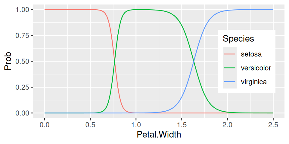
Code
xgrid |>
  modelr::add_predictions(model = fit, var = "Species", type = "class") |>
  ggplot() + aes(x = Petal.Width, y = Species) +
  geom_jitter(data = iris, height = 0.1) +
  geom_line(color = 4, linewidth = 1)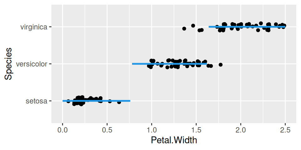
4.2.3 Ordinal
When the classes of nominal RV has some natural ordering, this can be used to make the multinomial logistic model more effective (less complex). The resulting ordered logit (or proportional odds logistic regression) model predicts the ratio of “at most” to “more than” probability, \[
\log\left(\frac{Pr[Y\leq k|X=x]}{Pr[Y>k|X=x]}\right) = b_{k1}-b_2x, \qquad \text{pre}\quad k=1,\ldots, K-1
\] - Each class has its own intercept but all share the parameter standing by \(X\).
- Parametrisation with the minus sign has its meaning for keeping the usual interpretation of \(b_2\).
In mtcars dataset, the number of cylinders is an example of ordinal RV. Let us predict its value conditional on displacement.
Code
dat |>
  ggplot() + aes(x = displacement, y = cylinders) +
  geom_boxplot(varwidth = TRUE, outlier.size = 0) +
  geom_jitter(height=0.1)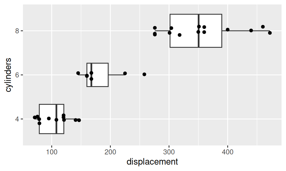
Code
fit <- dat |>
  dplyr::mutate(cylinders = ordered(cylinders, c("4","6","8"))) |>
  MASS::polr(cylinders ~ displacement, data=_)
fit
Call:
MASS::polr(formula = cylinders ~ displacement, data = dplyr::mutate(dat,
cylinders = ordered(cylinders, c("4", "6", "8"))))
Coefficients:
displacement
0.4443344
Intercepts:
4|6 6|8
64.9643 118.0268
Residual Deviance: 3.924663
AIC: 9.924663
Warning: did not converge as iteration limit reachedCode
xgrid <- data.frame(displacement = seq(70, 480, length.out = 100))

cbind(xgrid,
      predict(fit, newdata = xgrid, type="probs")
      ) |>
  tidyr::pivot_longer(cols = -displacement,
                      names_to = "cylinders", values_to = "Prob"
                      ) |>
  ggplot() + aes(x = displacement, y = Prob, color = cylinders, group = cylinders) +
  geom_line() +
  theme(legend.position = c(0.85,0.5))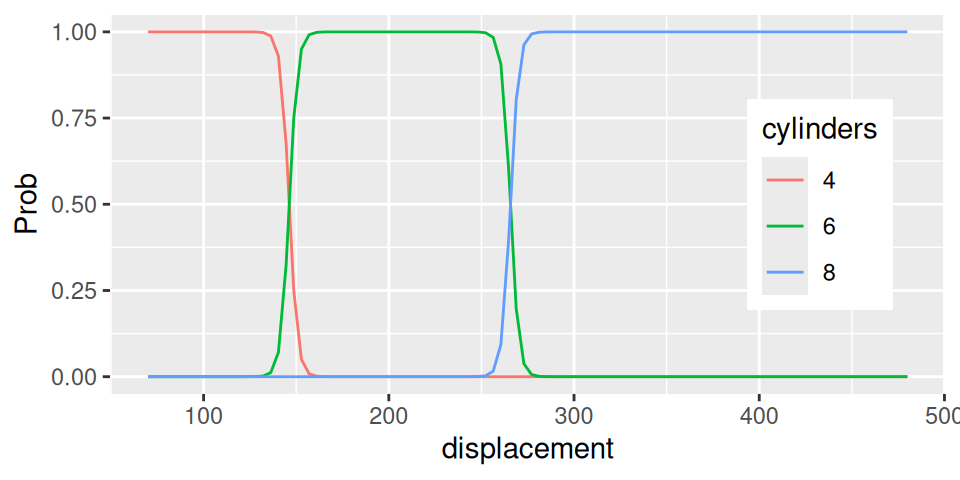
Code
xgrid |>
  modelr::add_predictions(model = fit, var = "cylinders", type = "class") |>
  ggplot() + aes(x = displacement, y = cylinders) +
  geom_jitter(data = dat, height = 0.1) +
  geom_line(color = 4, linewidth = 1)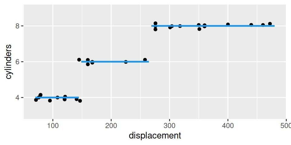
- Positive value of parameter \(b_2\) (0.4443) means that number of cylinders is an increasing function of displacement. In particular, raising displacement by one (inch3) would multiple the odds of lower classes (relative to higher classes) by \(e^{-0.444}=0.6\), i.e. odds get lower by 3/5.
- Let us predict number of cylinders for engine with 150 inch3 displacement: \[ \begin{split} logit\big(Pr[cyl\leq 4|disp=150]\big) &= 65.0 - 0.444\cdot150 = -1.6 \\ Pr[cyl\leq 4|disp=150] &= \frac{e^{-1.6}}{1+e^{-1.6}} = 0.168 \\ Pr[cyl\leq 6|disp=150] &= \frac{e^{118.0-0.444\cdot150}}{1+e^{118.0-0.444\cdot150}} \approx 1 \end{split} \] then class probabilities are \[ \begin{split} Pr[cyl = 4|disp=150] &= Pr[cyl \leq 4|disp=150] = 0.168 \\ Pr[cyl = 6|disp=150] &= Pr[cyl \leq 6|disp=150] - Pr[cyl \leq 4|disp=150] = 0.832 \\ Pr[cyl = 8|disp=150] &= 1 - Pr[cyl \leq 6|disp=150] \approx 0 \end{split} \] thus \[ E[cyl|disp=150]=6 \text{ cylinders}. \]
4.2.4 Generative methods
Logistic regression is a discriminative classification method because conditional distribution of response is modeled directly. On the other hand, generative methods such as linear (and quadratic) discriminant analysis or Naive Bayes describe probability distribution of predictors for each value of response.
- Let \(\pi_k \equiv Pr[Y=k]\), i.e an unconditional probability that randomly chosen observation belongs to class \(k\). So-called prior.
- Let function \(f_k(X)\) denote either PMF (if \(X\) is discrete) or PDF (\(X\) is continuous). Its value is large, if \(X\approx x\) for an observation from \(k\)-th class, and small if values of \(X\) are far from \(x\).
- Then, using Bayes theorem we can calculate (the so-called) posterior probability \[ Pr[Y=k|X=x] = \frac{\pi_k f_k(x)}{\sum_{l=1}^K \pi_l f_l(x)}. \]
So, instead of direct estimation of \(Pr[Y=k|X=x]\) (as in discriminative approach) it is enough to estimate \(\pi_k\), \(f_k\) and insert them to the above formula.
- Estimate of prior probability is simply a ratio of class specific sample size to total number of observations, i.e., \(\pi_k=\frac{n_k}{n}\).
- Estimation of \(f_k\) is far more challenging. To get it in a reasonable time and for required dimension, we need simplifying assumptions.
For example, linear and quadratic discriminant analysis assumes normal distribution for predictor \(X\), i.e., \[ f_k(x) = \frac{1}{\sqrt{2\pi}\sigma_k}\exp\left(-\frac{(x-\mu_k)^2}{2\sigma_k^2}\right) \] where \(\mu_k\) abd \(\sigma_k^2\) are mean value and variance in \(k\)-th class.
Linear discriminant analysis (LDA) further assumes equal variances across classes, i.e. \(\sigma_1=\ldots=\sigma_K=\sigma\). Applying Bayes theorem we get a formula which is unnecessarily complex for classification task and can be simplified to the so-called discriminant functions \(\delta_k\) that preserve mutual proportionality of the posterior probabilities, \[ \delta_k(x) = x\frac{\mu_k}{\sigma^2} - \frac{\mu_k^2}{2\sigma^2} + \ln\pi_k. \] Such a discriminant functions are linear in variable \(x\).
Things get more complicated in higher dimensions. In that case LDA assumes also equal covariances across classes. Moreover, thanks to normality the estimation is still quite fast.
However, if normality does not suit well to the application, one may opt for another generative method frequently used with multiple predictors: Naive Bayes classificator assumes no special type of distribution but to ease estimation of joint density it assumes independence among predictors \(X_1,\ldots,X_p\). Consequently, the joint density is given simply as product of marginal densities, i.e., \[ f_k(\vec{x}) = f_{k1}(x_1)\times f_{k2}(x_2)\times\ldots\times f_{kp}(x_p) \] Of course, the belief in independence is naive, but performance of this method is often surprisingly good, comparing to much more intricate models.
Code
dat |>
  ggplot() + aes(x = weight) +
  geom_density(aes(fill = transmission), adjust = 3, alpha = 0.5) +
  geom_rug(aes(color = transmission)) +
  theme(legend.position = c(0.85,0.85))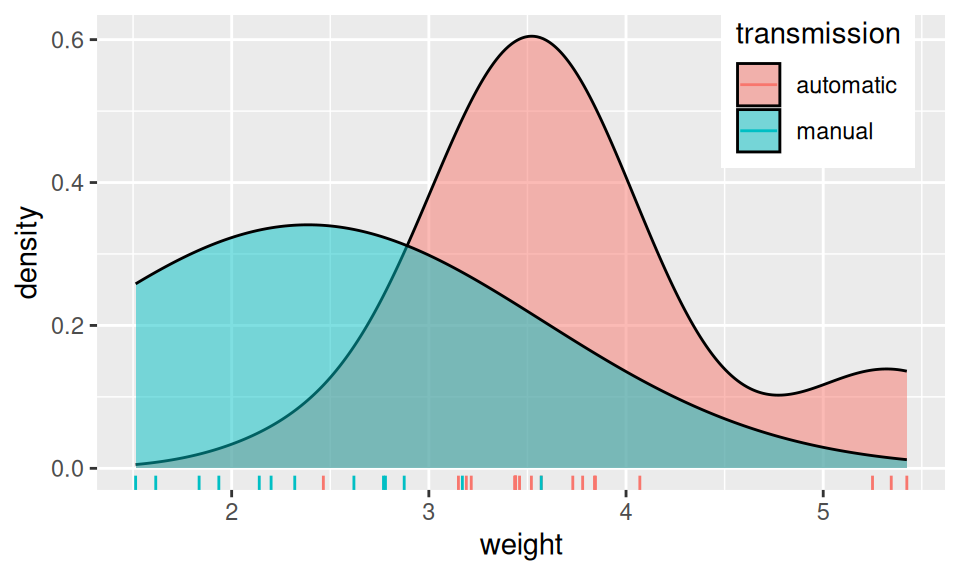
Code
fit <- MASS::lda(transmission ~ weight, dat)
fit
Call:
lda(transmission ~ weight, data = dat)
Prior probabilities of groups:
automatic manual
0.59375 0.40625
Group means:
weight
automatic 3.768895
manual 2.411000
Coefficients of linear discriminants:
LD1
weight 1.393632Code
sigma <- dat |>
  dplyr::summarise(s2 = var(weight), n = dplyr::n(), .by = transmission) |>
  dplyr::summarise(weighted.mean(s2, w = n-1)) |>
  as.numeric() |>
  sqrt()
ldfun <- function(x, mu, sig, pi) x*mu/sig^2 - (mu/sig)^2/2 + log(pi)
intersection <- mean(fit$means) - sigma^2 * diff(log(fit$prior))/diff(fit$means)
xgrid <- expand.grid(
  transmission = unique(dat$transmission),
  weight = modelr::seq_range(dat$weight, n = 50, expand = 0.2)
  ) |>
  dplyr::mutate(
    density = dnorm(weight, mean = fit$means[transmission], sd = sigma),
    discriminant = ldfun(weight, mu = fit$means[transmission], sig = sigma,
                         pi = fit$prior[transmission])
    )

posgrid <- data.frame(weight = unique(xgrid$weight)) |>
  (\(x) cbind(x, predict(fit, newdata = x)$posterior))() |>
  tidyr::pivot_longer(automatic:manual, names_to = "transmission", values_to = "posterior")

dplyr::left_join(xgrid, posgrid, by = c("weight", "transmission")) |>
  tidyr::pivot_longer(c(density, posterior, discriminant),
                      names_to = "fun", values_to = "value",
                      names_transform = forcats::as_factor
  ) |>
  ggplot() + aes(x = weight, y = value, color = transmission) +
  geom_line(linewidth = 1) +
  facet_grid(rows = vars(fun), scales = "free_y") +
  geom_vline(xintercept = intersection, linetype = 2) +
  theme(legend.position = c(0.87,0.1))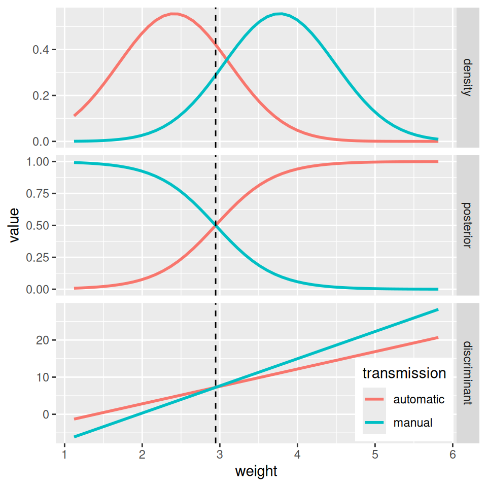
Code
data.frame(weight = unique(xgrid$weight)) |>
  dplyr::mutate(transmission = predict(fit, newdata = dplyr::cur_data())$class) |>
  ggplot() + aes(x = weight, y = transmission) +
  geom_jitter(data = dat, height = 0.05) +
  geom_line(color = 4, linewidth = 1)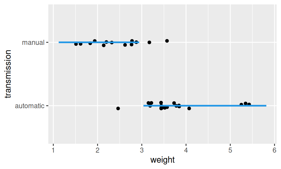
4.3 References
- van den Berg, S.M., 2022. Analysing data using linear models.
- Dalpiaz, D. 2018. Applied Statistics with R
- Navarro, D. 2018. Learning Statistics with R