1 Random variable and distributions of probability

Modified

March 19, 2025

Code

# load additional packages
library(ggplot2)

1.1 Motivation

When analyzing data, we

look for patterns,
use a sample to make an inference about the whole,

with the tools provided by probability theory and mathematical statistics.

Good knowledge helps to minimize unintentional misuse.

Example (cars)

First 10 observations from mtcars dataset:

Code

mtcars |> 
  tibble::rownames_to_column("model") |> 
  head(10) |> 
  pander::pander(split.tables = Inf)

model	mpg	cyl	disp	hp	drat	wt	qsec	vs	am	gear	carb
Mazda RX4	21	6	160	110	3.9	2.62	16.46	0	1	4	4
Mazda RX4 Wag	21	6	160	110	3.9	2.875	17.02	0	1	4	4
Datsun 710	22.8	4	108	93	3.85	2.32	18.61	1	1	4	1
Hornet 4 Drive	21.4	6	258	110	3.08	3.215	19.44	1	0	3	1
Hornet Sportabout	18.7	8	360	175	3.15	3.44	17.02	0	0	3	2
Valiant	18.1	6	225	105	2.76	3.46	20.22	1	0	3	1
Duster 360	14.3	8	360	245	3.21	3.57	15.84	0	0	3	4
Merc 240D	24.4	4	146.7	62	3.69	3.19	20	1	0	4	2
Merc 230	22.8	4	140.8	95	3.92	3.15	22.9	1	0	4	2
Merc 280	19.2	6	167.6	123	3.92	3.44	18.3	1	0	4	4

Example (floods)

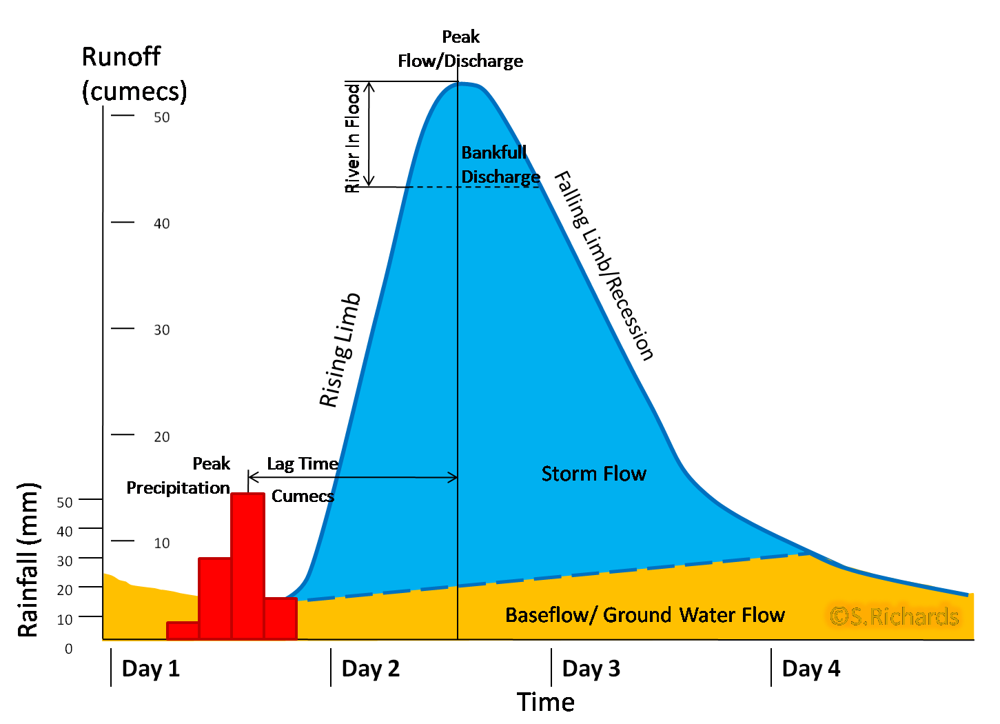
Code

read.csv("data/QmaxVolumeTime_anual(5180).csv") |>
  setNames(c("Year", "Peak", "Volume", "Duration")) |>
  dplyr::select(-Duration) |>
  tidyr::pivot_longer(cols = c(Peak, Volume), 
                      names_to = "variable", values_to = "value") |>
  ggplot() + aes(x = Year, y = value) + 
  geom_point() + geom_line(linetype = "dotted") + 
  facet_grid(rows = vars(variable), scales = "free_y") +
  #theme(text = element_text(size = 15)) +
  ylab("")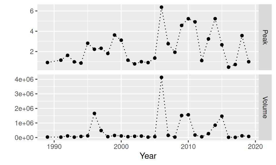

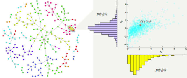
Example (system of RV)

1.2 Random variable

Random variable \(X\) is a function that projects a random event to numeric or some other formal value. Mostly we deal with numerical (i.e. quantitative) random variables (RV), later we show, that also the non-numerical ones (i.e. nominal, qualitative) are important.

Each value of RV may happen with some probability, e.g., if a person walking by is taken as a statistical unit (who I observe) than his height is a random event that may be mapped by numerical RV as “height in centimeters”, which formally attain values from \(\mathbb{R}^+\), in reality just from the interval, say, (30, 250), but also may be mapped by a nominal RV with three values: “low”, “normal”, “tall”. The probability, that the accidental passer-by will be tall, is intuitively smaller than the probability that he will be of normal height.

According to the range (image) of RV, denoted \(ran(X)\), we distinguish a variable to be either discrete or continuous.

The set of probabilities for all values of RV is called distribution of probability and it fully defines the RV. Distribution can be characterized by

probability mass function (PMF, in case of discrete RV),
probability density function (PDF, continuous RV) or
cumulative distribution function (CDF, for any RV with ordered values).

PMF represents probability of certain discrete value \(x\), formally \[ p(x) = Pr(X=x), \] while CDF represents probability that \(X\) will not exceed certain value, i.e. \[ F(x) = Pr(X\leq x) = \begin{cases} \sum\limits_{i:\ x_i\leq x} p(x_i) & \text{for discrete } X \\ \int\limits_{-\infty}^x f(t)dt & \text{for continuous } X \end{cases} \] where \(f\) denotes PDF and \(\{x_i\}\) is a set of all values of \(X\).

If we know probability distribution, we are able to calculate any characteristics of RV. Those are usually the first moments such as mean, variance, skewness and kurtosis which are measures of location, variability, asymmetry and (in a sense) extremeness, respectively. In particular the first two are given by the following formulas,

mean (expected value, first raw moment) \[ E[X] = \sum_i x_ip(x_i) \quad\text{or}\quad E[X] = \int_{ran(X)} tf(t)dt, \]
variance (second central moment), generally defined as \[ var(X) = E[(X-E[X])^2] \] which – in terms of probability mass/density – means \[ \begin{split} var(X) &= \sum_i (x_i-E[X])^2p(x_i) \qquad\text{or} \\ var(X) &= \int_{ran(X)} (t-E[X])^2f(t)dt. \end{split} \]

Besides moments, any quantitative or discrete ordinal RV can also be characterized by quantiles \(q_p\) associated with probability \(p\) through relation \[ Pr(X\leq q_p) = p \] A well known example is median (\(q_{0.5}\), the 50%-quantile), quartiles (\(q_0,q_{1/4},q_{1/2},q_{3/4},q_1\)), or their spread measure given by interquartile range (IQR = \(q_{3/4} - q_{1/4}\)).

Distribution of nominal RV is usually represented by mode, a value with the highest probability.

1.3 Distribution of discrete RV

1.3.1 Bernoulli

If a random variable \(X\) can attain only two values, say \(\{M, F\}\), than it follows Bernoulli distribution with parameter \(p\). The parameter represents probability, that in a random trial one of the values (a chosen one) will be observed.

Probability mass function is defined by relation

\[ p(x) = \begin{cases} p & \quad\text{if}\quad x=M \\ 1-p & \quad\phantom{a}\quad x=F\end{cases} \]

Code

data.frame(x = forcats::as_factor(c("M","F")), PMF =  c(2/3, 1/3)) |> 
  ggplot() + aes(x = x, y = PMF) +
  geom_point() + geom_linerange(aes(ymin = 0, ymax = PMF)) +
  scale_y_continuous(breaks=c(0,0.33,0.67,1), limits = c(0,1))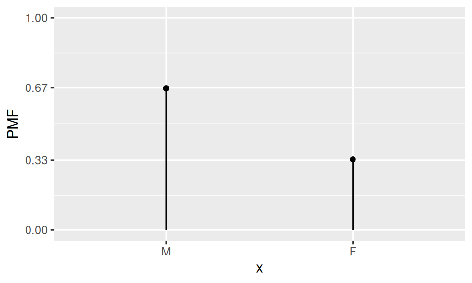

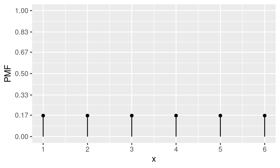
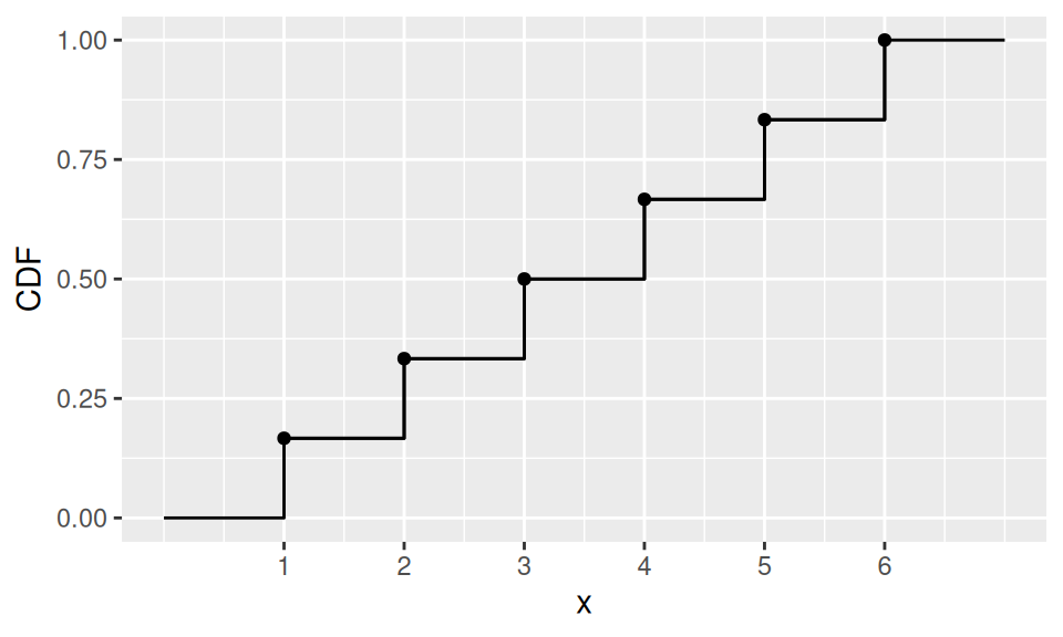
1.3.2 Uniform

If a random variable \(X\) can attain more than two values and all of them with the same probability, then \(X\) follows Uniform distribution. The probability mass function is constant, i.e. \[ p(x) = \frac1{card(X)} \] while it has no mode.

A well known example is rolling a dice with \(X\) representing the outcome (symbol or number of dots on the uppermost side).

Code

n <- 6
dat <- data.frame(x = 1:n) |> 
  dplyr::mutate(PMF = 1/n, 
                CDF = cumsum(PMF)
                ) 
dat |> 
  ggplot() + aes(x = x, y = PMF) +
  geom_point() + geom_linerange(aes(ymin = 0, ymax = PMF)) +
  scale_x_continuous(breaks=1:n) + 
  scale_y_continuous(breaks=round(0:6/6,2), limits = c(0,1))
dat |>
  ggplot() + aes(x = x, y = CDF) +
  geom_point() + geom_step() +
  scale_x_continuous(breaks=1:n) +
  geom_path(data = data.frame(
    x = c(0,rep(dat$x,each=2),7), 
    CDF = c(0,0,rep(dat$CDF,each=2))
    ))

1.3.3 Binomial

If Bernoulli trial is repeated \(n\)-times, and \(X\) is set as the number of desired outcomes, then \(X\) follows Binomial distribution with parameters \(p\) and \(n\). Formally we write \(X\sim B(n,p)\).

The probability mass function is defined by \[ p(x) = \binom{n}{x}p^x(1-p)^{n-x} \] and \(x\in\{0,1,\ldots,n\}\). Mean value and variance are also well-defined, \[ E[X] = np, \qquad var(X) = np(1-p). \] Example

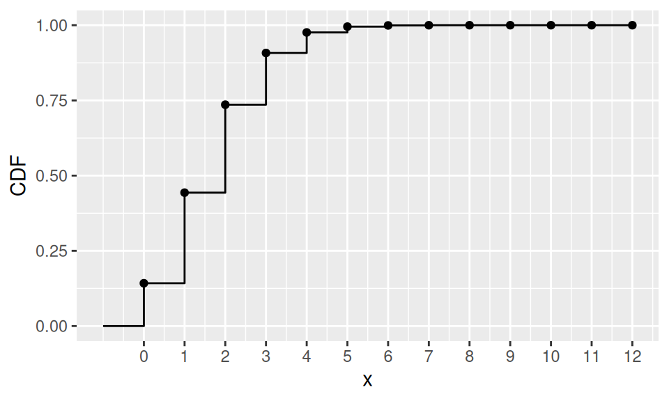
According to a bank observations 15% of customers, who have a payment card, have asked at least once for blocking the card. Now, given a sample of 12 card holders, what is the probability, that
1. at most
2. exactly
3. at least
one of them will use the bank service? Also show PMF, CDF and find mean, median and mode.

Code

p <- 0.15
n <- 12
dat <- data.frame(x = 0:n) |> 
  dplyr::mutate(PMF = dbinom(x, size = n, prob = p), 
                CDF = cumsum(PMF)
                ) 
dat |> 
  ggplot() + aes(x = x, y = PMF) +
  geom_point() + geom_linerange(aes(ymin = 0, ymax = PMF)) +
  scale_x_continuous(breaks=0:n)
dat |>
  ggplot() + aes(x = x, y = CDF) +
  geom_point() + geom_step() +
  scale_x_continuous(breaks=0:n) +
  geom_path(data = data.frame(x = c(-1,0,0), CDF = c(0,0,dat$CDF[1])))
with(dat,
     list(probability = c("Pr(X≤1)" = CDF[x==1], "Pr(X=1)" = PMF[2], "Pr(X≥1)" = 1-CDF[1]) |> round(3),
          location = c("E(X)" = sum(x*PMF), "Me(X)" = qbinom(0.5,n,p), "Mo(X)" = x[which.max(PMF)])
          )
     ) |> 
  pander::pander()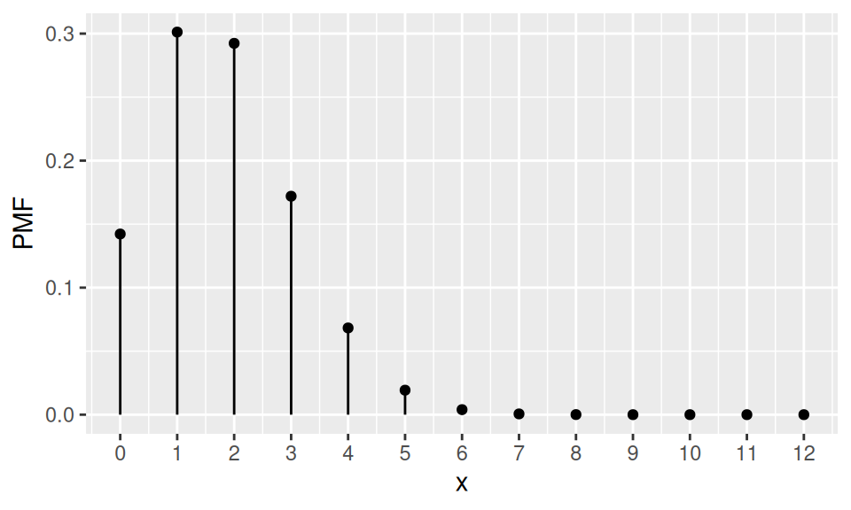

probability:

Pr(X≤1) Pr(X=1) Pr(X≥1)

0.443 0.301 0.858
location:

E(X) Me(X) Mo(X)

1.8 2 1

Pr(X≤1)	Pr(X=1)	Pr(X≥1)
0.443	0.301	0.858

E(X)	Me(X)	Mo(X)
1.8	2	1

1.3.4 Poisson

If the number of trials grows (\(n\to\infty\)) and probability of single success decreases (\(p\to0\)), such that the expected value remains the same (\(np=\lambda\)), then the Binomial distribution can be approximated by Poisson distribution with the parameter \(\lambda\) (rate). The PMF is defined by \[ p(x) = \frac{\lambda^xe^{-\lambda}}{x!},\qquad \lambda\in(0,\infty) \] and its mean is equal to variance, \(E[X]=var(X)=\lambda\).
Thus the Poisson distribution can be applied to the systems with a large number of possible events, each of which is rare.

Example

There are 2000 components in a machine. Failure probability of single component is equal to 0.005. If the random variable \(X\) represents number of broken components, what is the probability that more than 10 components will fail?

Code

p <- 0.005
n <- 2000
lambda <- n*p
dat <- data.frame(x = 0:(3*lambda)) |> 
  dplyr::mutate(PMF = dpois(x, lambda), 
                CDF = cumsum(PMF)
                ) 
dat |> 
  ggplot() + aes(x = x, y = PMF) +
  geom_point() + geom_linerange(aes(ymin = 0, ymax = PMF))
dat |>
  ggplot() + aes(x = x, y = CDF) +
  geom_point() + geom_step() +
  geom_path(data = data.frame(x = c(-1,0,0), CDF = c(0,0,dat$CDF[1])))
c("λ" = lambda, "Pr(X>10)" = 1 - ppois(10, lambda)) |> round(3)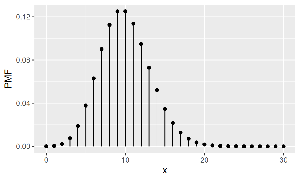

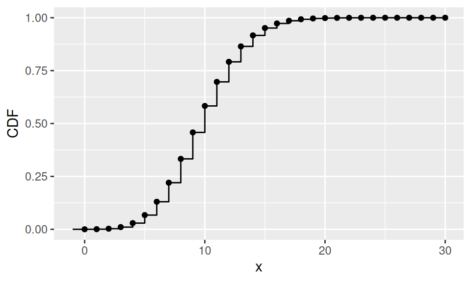
       λ Pr(X>10) 
  10.000    0.417

1.4 Distribution of continuous RV

1.4.1 Uniform

Discrete uniform distribution has also its counterpart among continuous distributions. Whenever \(X\) follows uniform distribution with parameters (limits) \(a,b\), i.e., \(X\sim U(a,b)\), its probability density function is defined as \[ f(x) = \frac1{b-a} \] Mean value (also median) is obviously a simple average of the limits, \(E[X]=\frac{a+b}{2}\), while variance is given by \(var(X)=\frac1{12}(b-a)^2\). Again, there is no single mode.

This is, for example, the distribution of waiting time for a bus, if its inter-arrival period is \((b-a)\).

Example

Find a probability, that we will wait 2 to 6 minutes for our bus, if it is departed in 10min intervals.

Code

b <- 10
a <- 0
ba <- b-a
dat <- data.frame(x = c(a-ba/5, a, a, b, b, b+ba/5)) |> 
  dplyr::mutate(PDF = c(0,0,dunif(c(a,b), a, b), 0, 0), 
                CDF = punif(x, a, b),
                linegroup = rep(1:3, each=2)
                )
dat1 <- dat |> 
  dplyr::slice(2:5) |> 
  dplyr::mutate(linegroup = c(1,1,2,2))
dat2 <- data.frame(x = c(2,6)) |> 
  dplyr::mutate(CDF = punif(x, a, b))

dat |> 
  ggplot() + aes(x = x, y = PDF, group = linegroup) +
  geom_line() + 
  geom_line(data = dat1, linetype = 2) +
  scale_y_continuous(breaks=range(dat$PDF)) + 
  scale_x_continuous(breaks=seq(0,10,2)) +
  geom_rect(xmin = dat2$x[1], xmax = dat2$x[2], 
            ymin = 0, ymax = 1/ba, alpha = 0.05)
dat |>
  ggplot() + aes(x = x, y = CDF) +
  geom_line() + 
  scale_x_continuous(breaks=seq(0,10,2)) +
  scale_y_continuous(breaks=punif(seq(0,10,2),a,b)) +
  geom_linerange(aes(ymax = CDF), data = dat2, ymin=0, linetype = 3) +
  geom_linerange(aes(xmax = x), data = dat2, xmin=dat$x[1], linetype = 3, orientation = "y")
c("E[X]" = mean(c(a,b)), "var(X)" = ba^2/12, "Pr(2<X≤6)" = diff(dat2$CDF)) |> round(1)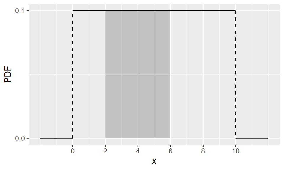

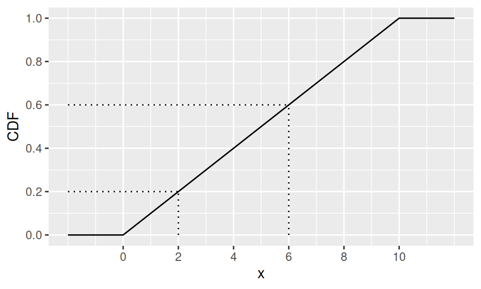
     E[X]    var(X) Pr(2<X≤6) 
      5.0       8.3       0.4

1.4.2 Normal (Gaussian)

Back in the Binomial distribution case, if we let \(n\) (the number of Bernoulli trials) go to infinity, the distribution of the random variable (which represented the number of successful trials) would become normal with parameters \(\mu = np\) (mean) and \(\sigma^2 = np(1-p)\) (variance). The density function is given by \[ f(x) = \frac1{\sqrt{2\pi}\sigma}\exp\left\{-\frac{x-\mu}{2\sigma}\right\}, \] where \(\sigma\) is the so-called standard deviation.

A special case, standard normal distribution, is frequently used in statistics. It is the distribution of the standardized (centered and rescaled) random variable \(Z=\frac{X-\mu}{\sigma}\).

Code

# parameters
p <- 0.15
n <- 100
mu <- n*p
sigma <- sqrt( n*p*(1-p) )
# data to plot
datB <- data.frame(x = 0:(n*p*2.2)) |> 
  dplyr::mutate(binomial = dbinom(x, size = n, prob = p)) 
datN <- data.frame(x = seq(0,n*p*2.2,0.1)) |> 
  dplyr::mutate(normal = dnorm(x, mu, sigma))
# plots
ggplot() + aes(x = x) +
  geom_point(aes(y = binomial, color = "binomial"), 
             data = datB, shape = 16) + 
  geom_line(aes(y = normal, color = "normal"), 
            data = datN, linetype = 1) +
  scale_color_manual(values = c(binomial = 1, normal = 2),
                     labels = c(binomial = "B(100,0.15)", normal = "N(15,3.6²)")
                     ) +
  guides(color = guide_legend(
    override.aes = list(shape = c(16,NA), linetype = c(NA, 1)),
    title = "distribution")) +
  theme(legend.position = c(0.8, 0.8)) +
  ylab("PMF/PDF")
# standardization
dat <- data.frame(x = seq(-3*sigma, mu + 3*sigma, 0.1)) |> 
  dplyr::mutate("N(15,3.6²)" = dnorm(x, mu, sigma),
                "N(0,3.6²)" = dnorm(x, 0, sigma),
                "N(0,1)" = dnorm(x)
                ) |> 
  tidyr::pivot_longer(-x, names_to = "distribution", values_to = "PDF")
dat |> 
  ggplot() + aes(x = x, y = PDF, color = distribution) +
  geom_line() + 
  scale_color_manual(values = 4:2) + 
  guides(color = guide_legend(reverse = TRUE)) +
  theme(legend.position = c(0.8, 0.8))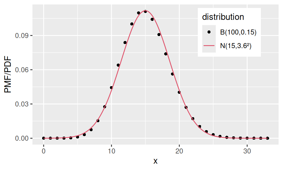

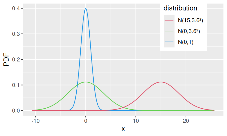
If two random variables \(X_1,X_2\) follow normal distribution, i.e., \(X_1\sim N(\mu_1,\sigma_1^2)\) and \(X_2\sim N(\mu_2,\sigma_2^2)\), then their linear combination \(Y = aX_1 + bX_2 + c\) also follows normal distribution, \(Y \sim N(a\mu_1+b\mu_2+c, a^2\sigma_1^2 + b^2\sigma_2^2)\).

1.4.3 Log-normal

If \(X\sim N(\mu,\sigma^2)\) then random variable \(Y=e^X\) follows log-normal distribution, \(Y\sim LN(\mu,\sigma^2)\).

In nature a lot of random variables follows a distribution that is close to log-normal (i.e., positive-valued). Thus by taking their logarithm it is possible to turn their distribution into approximately normal, which enables one to use wast amount of methods available in statistics that require normality.

Code

dat <- data.frame(x = seq(-3, 5, 0.01)) |> 
  dplyr::mutate("N(0,1)" = dnorm(x),
                "LN(0,1)" = dlnorm(x)
                ) |> 
  tidyr::pivot_longer(-x, names_to = "distribution", values_to = "PDF")
dat |> 
  ggplot() + aes(x = x, y = PDF, color = distribution) +
  geom_line() + 
  scale_color_manual(values = c(6,4)) + 
  guides(color = guide_legend(reverse = TRUE)) +
  theme(legend.position = c(0.8, 0.8))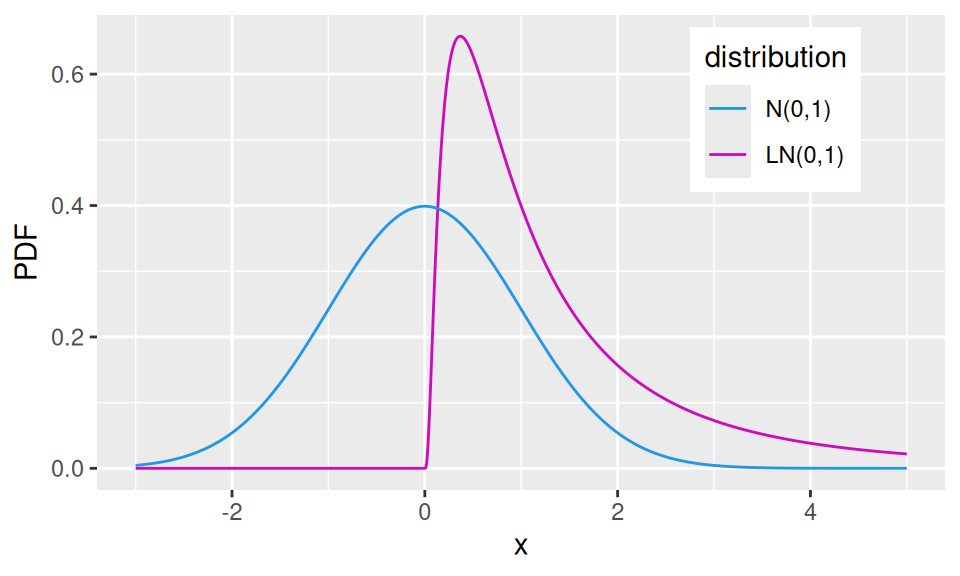

1.4.4 \(\chi^2\) (chi-squared) distribution

If \(X_1,X_2,\ldots X_n\) come from standard normal \(N(0,1)\), then \(Y=X_1^2+X_2^2+\ldots+X_n^2\) follows chi-square(d) distribution with (parameter) \(n\) degrees of freedom, i.e., \(Y\sim\chi^2(n)\). We also get mean value \(E[Y]=n\) and variance \(var(Y)=2n\).

Code

dat <- data.frame(x = seq(-3, 5, 0.01)) |> 
  dplyr::mutate("N(0,1)" = dnorm(x),
                "χ²(3)" = dchisq(x, 3),
                "χ²(4)" = dchisq(x, 4),
                ) |> 
  tidyr::pivot_longer(-x, names_to = "distribution", values_to = "PDF")
dat |> 
  ggplot() + aes(x = x, y = PDF, color = distribution) +
  geom_line() + 
  scale_color_manual(values = c(4,3,2)) +
  theme(legend.position = c(0.8, 0.75))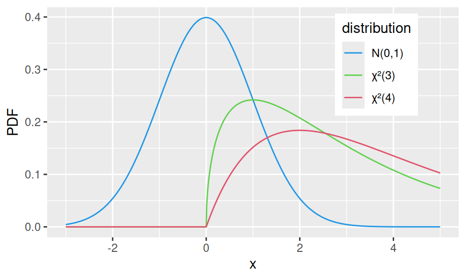

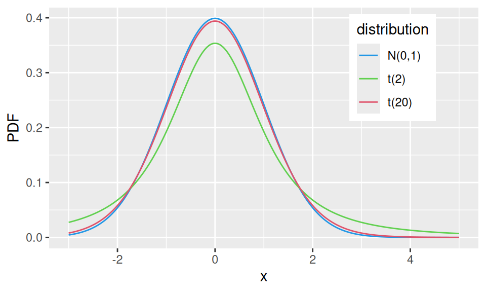
1.4.5 t-distribution

If \(X_1\sim N(0,1)\) and \(X_2\sim\chi^2(n)\) then \(Y\sim\frac{X_1}{\sqrt{X_2/n}}\) follows the Student’s t-distribution with (parameter) \(n\) degrees of freedom, i.e., \(Y\sim t(n)\) for which we have the mean value \(E[Y]=0\) and variance \(var(X)=\frac{n}{n-2}\).

Code

dat <- data.frame(x = seq(-3, 5, 0.01)) |> 
  dplyr::mutate("N(0,1)" = dnorm(x),
                "t(2)" = dt(x, 2),
                "t(20)" = dt(x, 20),
                ) |> 
  tidyr::pivot_longer(-x, names_to = "distribution", values_to = "PDF")
dat |> 
  ggplot() + aes(x = x, y = PDF, color = distribution) +
  geom_line() + 
  scale_color_manual(values = c(4,3,2)) +
  theme(legend.position = c(0.8, 0.75))