3 Testing statistical hypotheses
Code
# load additional packages
library(ggplot2)

# elementary transformations before analysis is applied
dat <- mtcars |>
  dplyr::transmute(
    mileage = mpg,
    cylinders = as.factor(cyl),
    horsepower = hp,
    displacement = disp,
    weight = wt,
    transmission = dplyr::recode(am, `0` = "automatic", `1` = "manual")
    )
n <- nrow(dat)
3.1 Fundamental concepts
Notes from Navarro (2018):
In its most abstract form, hypothesis testing is really a very simple idea: the researcher has some theory about the world, and wants to determine whether or not the data actually support that theory. However, the details are messy, and most people find the theory of hypothesis testing to be the most frustrating part of statistics.
A statistical hypothesis test is a test of the statistical hypothesis, not the research hypothesis. If your study is badly designed, then the link between your research hypothesis and your statistical hypothesis is broken. Check the examples on page 328.
The “null” hypothesis, H0 corresponds to the exact opposite of what I want to believe. The goal of a hypothesis test is not to show that the alternative hypothesis is (probably) true; the goal is to show that the null hypothesis is (probably) false.
Useful analogy: The null hypothesis is the defendant, the researcher is the prosecutor, and the statistical test itself is the judge. There is a presumption of innocence: the null hypothesis is deemed to be true unless you, the researcher, can prove beyond a reasonable doubt that it is false. You are free to design your experiment however you like (within reason, obviously!), and your goal when doing so may be to maximise the chance that the data will yield a conviction… for the crime of being false. The catch is that the statistical test sets the rules of the trial, and those rules are designed to protect the null hypothesis … the chances of a false conviction are guaranteed to be low.
The goal behind statistical hypothesis testing is NOT to eliminate errors, but to minimise them.
A statistical test really doesn’t prove that a hypothesis is true or false.
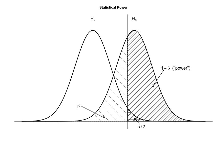
If we reject a null hypothesis that is actually true, then we have made a type I error (α). On the other hand, if we retain the null hypothesis when it is in fact false, then we have made a type II error (β).
It is “better that ten guilty persons escape than that one innocent suffer” (Blackstone). A statistical test is pretty much the same: the single most important design principle of the test is to control the probability of a type I error, to keep it below some fixed probability (significance level, size of the test).
Power of the test is the probability (1 - β) with which we reject a null hypothesis when it really is false.
Notice the asymmetry here … the tests are designed to ensure that the α level is kept small, but there’s no corresponding guarantee regarding β.
(To paraphrase) it is “better to retain 10 false null hypotheses than to reject a single true one”. To be honest, there are situations where it makes sense, and situations where it doesn’t. But it’s how the tests are built.
A quantity (that we can calculate by looking at our data) that helps us to make a decision about whether to believe that the null hypothesis is correct, or to reject the null hypothesis in favour of the alternative, is called test statistic.
Having chosen a test statistic, the next step is to state precisely which values of the test statistic would cause us to reject the null hypothesis, and which values would cause us to keep it. In order to do so, we need to determine what the sampling distribution of the test statistic would be if the null hypothesis were actually true.
The question that remains is this: exactly which values of the test statistic should we associate with the null hypothesis, and exactly which values go with the alternative hypothesis? The answer introduces the concept of a critical region (rejection region): it is those values of test statistic that would lead us to reject null hypothesis (very small or very big values, covering α·100% of the sampling distribution of test statistic). Critical region consists of the most extreme values, known as the tails of the distribution. The edges of the critical region are often referred to as the critical values.
A lot of modern readers get very confused when they start learning statistics, because they think that a “significant result” must be an important one. It does not mean that at all. All that “statistically significant” means is that the data allowed us to reject a null hypothesis.
There are two somewhat different ways of interpreting a p-value, one proposed by Jerzy Neyman and the other by Ronald Fisher. (See also discussion in chapter 11.9.1, Neyman versus Fisher.)
- p-value is defined to be the smallest Type I error rate (α) that you have to be willing to tolerate if you want to reject the null hypothesis. (Neyman)
- Good critical region almost always corresponds to those values of the test statistic that are least likely to be observed if the null hypothesis is true. If this rule is true, then we can define the p-value as the probability that we would have observed a test statistic that is at least as extreme as the one we actually did get. In other words, if the data are extremely implausible according to the null hypothesis, then the null hypothesis is probably wrong. (Fisher)
- A third, and completely MISTAKEN approach is to refer to the p-value as “the probability that the null hypothesis is true”.
The one thing that you always have to do is say something about the p-value, and whether or not the outcome was significant. The reason (why not reporting just a p-value and let others decide) is that it gives the researcher a bit too much freedom. It’s hard to let go and admit the experiment didn’t find what you wanted it to find. And that’s the danger here. If we use the “raw” p-value, people will start interpreting the data in terms of what they want to believe, not what the data are actually saying… and if we allow that, well, why are we bothering to do science at all? According to this view, you really must specify your α value in advance.
A secondary goal of hypothesis testing is to try to minimise β, the Type II error rate, or equally to maximise the power of the test (1-β). A Type II error occurs when the alternative hypothesis is true, but we are nevertheless unable to reject the null hypothesis. Ideally, we’d be able to calculate a single number β that tells us the Type II error rate, in the same way that we can set α = 0.05 for the Type I error rate. However, β depends on the true value of parameter which may be anything from the range specified by alternative hypothesis. To see all values of (1-β) a power function can be plotted. If the true state of the world is very different from what the null hypothesis predicts, then power will be very high; if similar to the null (but not identical) then the power of the test is going to be very low.
A statistic that quantify how “dissimilar” the true state of the world is to the null hypothesis (how big is the difference between the true population parameters and the parameter values assumed by the null hypothesis) is called a measure of effect size.
It is becoming more standard (slowly, but surely) to report some kind of standard measure of effect size along with the results of the hypothesis test. The hypothesis test itself tells you whether you should believe that the effect you have observed is real (i.e., not just due to chance); the effect size tells you whether or not you should care.
Not surprisingly, scientists are fairly obsessed with maximising the power of their experiments. We want our experiments to work, and so we want to maximise the chance of rejecting the null hypothesis if it is false. (And of course we usually want to believe that it is false!) One factor that influences power is the effect size.
Clever experimental design is one way to boost power; because it can alter the effect size. (Unfortunatelly, often, even the best design has small effect.) Another way is to increase sample size. In general, the more observations that you have available, the more likely it is that you can discriminate between two hypotheses.
3.2 Classification of tests
For most common statistical hypothesis there exist several statistical tests that differ by assumptions and the related power.
Let’s go through some basic classifications:
- If the sample comes from normal distribution, a parametric test has more power than a non-parametric one.
- According to the type of inequality stated by alternative hypothesis, the test is one-sided or two-sided.
- Tests concerning single random variable are so-called one-sample tests.
- For more than one sample, observations may come from the same object (paired, repeated measures) or not.
- The main classification relies on the type of RV involved: continuous, discrete ordinal, discrete nominal.
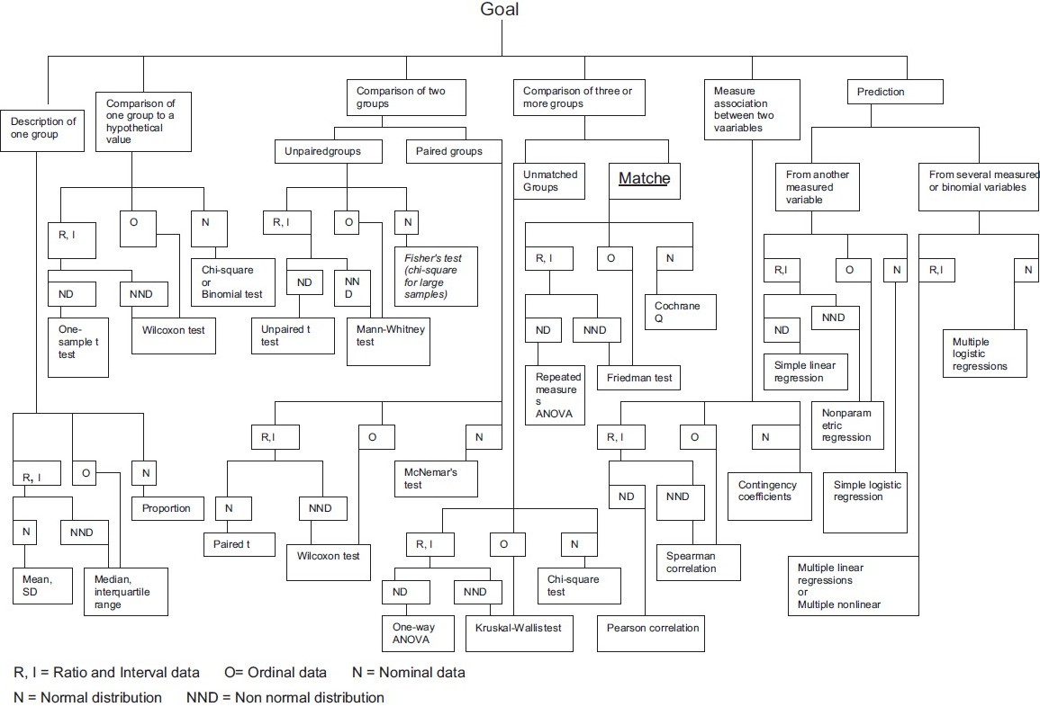
Several other flow charts for commonly used statistical tests can be found on internet (1, 2).
3.3 Single variable
From the variety of one-sample statistical tests, one selects the right test according to its purpose:
- parameters of a distribution
- proportion
- mean or median (one-sample t-test, Wilcoxon)
- variance
- type of distribution
- normality (Shapiro-Wilk, Jarque-Bera, …)
- general (\(\chi^2\), Kolmogorov-Smirnov, Anderson-Darling, Cramér-von Mises)
- assumptions
- outliers (Grubbs, Dixon)
- randomness/autocorrelation
A typical scenario for continuous random variable is to check randomness of a sample, normality of the RV (taking outliers into account), and then test hypothesis about location.
3.3.1 Parameters of a distribution
A binary random variable has a Bernoulli distribution with parameter \(p\), which we are interested in. Without loosing generality, let the variable attain values from the set \(\{0,1\}\). Given \(n\) such binary and mutually independent variables \(X_i\) (e.g. by repeating Bernoulli trials) the random variable
\[
Y=\frac1n\sum_{i=1}^n X_i
\] (i.e. proportion of “successes”) has mean value \(E[Y]=p\) and variance \(var(Y) = p(1-p)/n\). From central limit theorem for \(n\) large enough we know that \(Y\) follows normal distribution.
Let us test that the true parameter \(p\) is equal to some hypothetical value \(p_0\), i.e. \(H_0\colon p=p_0\), against \(H_1\colon p\neq p_0\). If \(H_0\) holds, then \(Y\) follows \(N\left(p_0,\frac{p(1-p)}{n}\right)\), or equivalently, \[ \frac{Y-p_0}{\sqrt{p(1-p)/n}}\sim N(0,1) \] Since \(p\) is not known, it may be approximated by an unbiased estimate from sample.
For example, a national car seller claims that two thirds of car models presently sold have automatic transmission.
Code
n <- nrow(dat)
phat <- sum(dat$transmission == "automatic") / n
p0 <- 2/3
sig <- sqrt(phat*(1-phat)/n)
c(TS = phat,
  qnorm(c(qL = 0.025, qU = 0.975), mean = p0, sd = sig),
  p.value = 2*pnorm(phat, mean = p0, sd = sig)
) |> round(3)
TS qL qU p.value
0.594 0.497 0.837 0.401 Code
sum(dat$transmission == "automatic") |>
  prop.test(n = nrow(dat), p = 2/3, correct = F)
    1-sample proportions test without continuity correction

data:  sum(dat$transmission == "automatic") out of nrow(dat), null probability 2/3
X-squared = 0.76562, df = 1, p-value = 0.3816
alternative hypothesis: true p is not equal to 0.6666667
95 percent confidence interval:
 0.4226002 0.7448037
sample estimates:
      p
0.59375
Based on the data we have at disposal, the null hypothesis \(H_0:p=\frac23\) can not be rejected.
With continuous variable \(X\) from normal distribution, one usually needs to verify a hypothesis, that its mean value \(\mu\) is equal to a hypothetical value \(\mu_0\) (either strictly, or at most, or at least). Knowing that average of normally distributed variables is normal with the same mean but smaller variance, test statistic of the so-called Student’s t-test defined by \[ TS = \frac{\hat\mu-\mu_0}{\frac{\hat\sigma}{\sqrt{n}}} \] follows t-distribution with \((n-1)\) degrees of freedom.
For instance, let us verify a statement, that cars have mean mileage no greater than 18 miles per gallon. Null hypothesis always includes equality, thus \(H_0\colon E[\text{mileage}]\leq18\)mpg.
Code
mu <- dat$mileage |> mean()
sig <- dat$mileage |> sd()
TS <- (mu - 18) / sig * sqrt(n)
c(mean = mu,
  TS = TS,
  qt(c(qL = 0, qU = 0.95), df = n-1),
  p.value = 1 - pt(TS, df = n-1)
) |> round(3)
mean TS qL qU p.value
20.091 1.962 -Inf 1.696 0.029 Code
dat$mileage |> t.test(mu = 18, alternative = "greater")
    One Sample t-test

data:  dat$mileage
t = 1.9622, df = 31, p-value = 0.02938
alternative hypothesis: true mean is greater than 18
95 percent confidence interval:
 18.28418      Inf
sample estimates:
mean of x
 20.09062
Based on the sample statistic and its distribution (under the null), we can conclude with 5% risk, that mean mileage is greater than 18 miles per galon.
If normality of \(X\) is not guaranteed, then mean value as a measure of location could be misleading. In that case, it is wise to reach for median and non-parametric tests for location such as Wilcoxon signed rank test.
Given a sample \(\{x_i\}_{i=1}^n\) and hypothetic measure of location \(m_0\) the test statistic \(W^+\) is calculated by formula \[
W^+ = \sum_{i=1}^n 1_{[0,\infty)}(d_i)R_i,
\] where \(d_i = x_i-m_0\), and \(R_i\) is rank of \(|d_i|\) (absolute value of \(d_i\)). The test statistic is bounded by values 0 (i.e, whole sample is smaller than \(m_0\)) and \(\frac{n(n+1)}{2}\) (sum of arithmetic series; each \(x_i\) is over \(m_0\)). Due to central limit theorem it holds that
\[
W^+\overset{a}{\sim}N\left(\frac{n(n+1)}{4},\frac{n(n+1)(2n+1)}{24}\right).
\]
To illustrate the matter, let us verify the hypothesis, that engine displacement is “overall” smaller than a half of its range, i.e. \(H_0\colon Me(displacement)\geq250\)inch3. We employ three approaches, first using asymptotic properties, then bootstrap method and finally a built-in method with continuity correction.
Code
c(mean = mean(dat$displacement),
  median = median(dat$displacement)
  ) |> signif(4)
mean median
230.7 196.3 Code
dat |>
  ggplot() + aes(x = displacement) +
  geom_histogram(aes(y = after_stat(density)), bins = 10,
                 color = "white", alpha = 0.5) +
  geom_rug() +
  geom_density()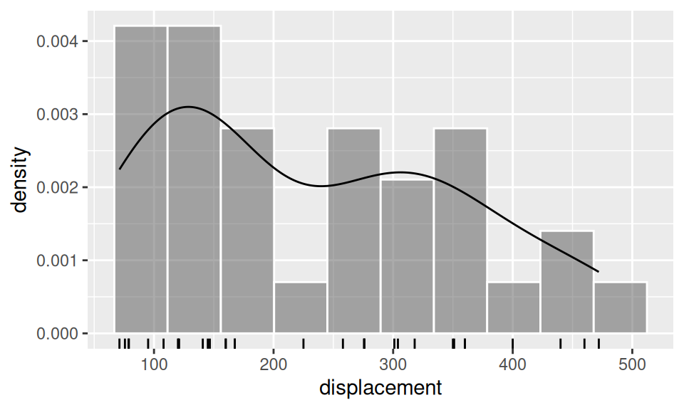
Code
# main function
wilcoxon.norm <- function(x, m0, H1 = c("two.sided", "less", "greater"), conf.level = 0.95) {
  n <- length(x)
  dif <- x - m0
  W <- sum( ifelse(dif>0,1,0)*rank(abs(dif)) )
  Wst <- (W - n*(n-1)/4) / sqrt(n*(n+1)*(2*n+1)/24)
  a <- 1 - conf.level
  quan <- switch(H1[1],
                 two.sided = qnorm(c(qL = a/2, qU = 1-a/2)),
                 less = qnorm(c(qL = a, qU = 1)),
                 greater = qnorm(c(qL = 0, qU = 1-a))
                 )
  pval <- switch(H1[1],
                 two.sided = 2 * min(pnorm(Wst), 1-pnorm(Wst)),
                 less = pnorm(Wst),
                 greater = 1 - pnorm(Wst)
                 )
c(W = W,
  Wst = Wst,
  quan,
  p.value = pval
)
}
# evaluation
results <- dat$displacement |> wilcoxon.norm(m0 = 250, H1 = "less")
# display numeric results
results |> signif(3)
W Wst qL qU p.value
215.000 -0.617 -1.640 Inf 0.269 Code
# show test statistic distribution
data.frame(Wst = seq(-3, 3, by=0.1)) |>
  ggplot() + aes(x = Wst) +
  geom_function(fun = dnorm) +
  geom_vline(xintercept = results["Wst"], linetype = 2) +
  ylab("density")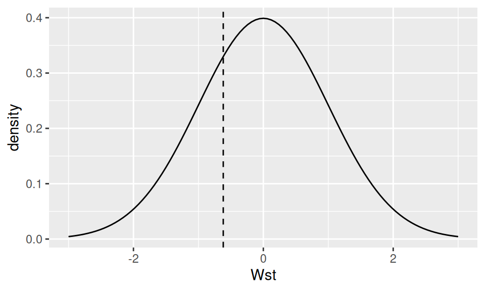
Code
# helper functions
wilcW <- function(x, m0) {
    dif <- x - m0
    sum( ifelse(dif > 0, 1, 0) * rank(abs(dif)) )
  }
wilcWsim <- function(n, N=1000) {
    replicate(N, runif(n)) |>
      apply(MARG = 2, FUN = wilcW, m0 = 1/2)
}
# main
wilcoxon.boot <- function(x, m0, H1 = c("two.sided", "less", "greater"),
                          conf.level = 0.95, N = 1000) {
  # initials
  n <- length(x)
  a <- 1 - conf.level
  # calculation
  W <- wilcW(x, m0)  # test statistic
  Wsim <- wilcWsim(n, N) # sample from H0 population
  quan <- switch(H1[1],
                 two.sided = quantile(Wsim, probs = c(qL = a/2, qU = 1-a/2),
                                      names = FALSE),
                 less = c(qL = quantile(Wsim, a, names = F), qU = n*(n+1)),
                 greater = c(qL = 0, qU = quantile(Wsim, 1-a, names = F))
  )
  pval <- switch(H1[1],
                 two.sided = 2 * min(sum(W>Wsim), sum(W<Wsim)) / N,
                 less = sum(Wsim < W) / N,
                 greater = sum(W < Wsim) /N
  )
  # output
  c(W = W,
    quan,
    p.value = pval
  )
}

# evaluation
dat$displacement |>
  wilcoxon.boot(m0 = 250, H1 = "less") |>
  signif(3)
W qL qU p.value
215.000 169.000 1060.000 0.166 Code
# visualization
data.frame(W = wilcWsim(n = nrow(dat))) |>
  ggplot() + aes(x = W) +
  geom_histogram(aes(y = after_stat(density)), bins = 10,
                 color = "white", alpha = 0.5) +
  geom_rug() +
  geom_density() +
  geom_vline(xintercept = results["W"], linetype = 2)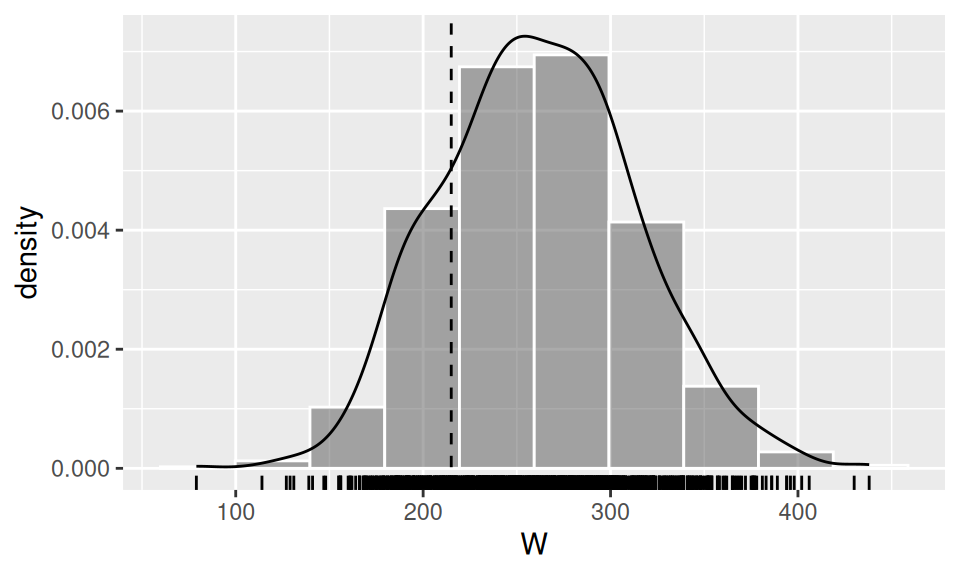
Code
dat$displacement |>
  wilcox.test(mu = 250, alternative = "less", exact=FALSE)
    Wilcoxon signed rank test with continuity correction

data:  dat$displacement
V = 215, p-value = 0.1822
alternative hypothesis: true location is less than 250
There is not enough evidence to reject \(H_0\), thus true median of population displacement could be equal to 250 cubic inches.
3.3.2 Type of distribution
As seen above, knowing the type of distribution – or at least whether normality is fulfilled – helps to choose between parametric and non-parametric methods.
To check, whether the sample could originate from a specific distribution, one can use general-purpose goodness-of-fit tests such as Chi-squared, Kolmogorov-Smirnov and Anderson-Darling test. If specifically a normal distribution is considered under \(H_0\), additional tests such as Jarque-Bera, Shapiro-Wilk and Lilliefors test are at disposal.
For example, let us test, whether number of cylinders comes from population with discrete uniform distribution defined on the set \(\{4,6,8\}\). First, take a look at empirical distribution (aka frequency table).
Code
tab <- dat$cylinders |> table(dnn = "cylinders")
tab
cylinders
4 6 8
11 7 14 Then use it in testing procedure which compares observed frequencies with theoretical ones.
Code
tab |> chisq.test() # discrete uniform is set by default
    Chi-squared test for given probabilities

data:  tab
X-squared = 2.3125, df = 2, p-value = 0.3147
Another example is checking normality of mileage. Parameters are estimated from the sample.
Code
shapiro.test(dat$mileage)
    Shapiro-Wilk normality test

data:  dat$mileage
W = 0.94756, p-value = 0.1229
In both cases, \(H_0\) should not be rejected with confidence 95%.
3.3.3 Assumptions
Many parametric statistical methods (if not all of them) assume randomness of the sample (meaning independent observations) and normality. Independence is achieved by randomization of the experiment and if in doubt, e.g. suspecting temporal dependence, one can perform e.g. turning point or runs test.
On the other hand, normality can be violated by one or few outliers. One rough method for outliers detection uses the 1.5 IQR rule. As a more formal alternative, Grubbs or Dixon test can be utilized.
3.4 Two variables
With two variables the main concern of statistical test is to draw conclusion about their dependence or, conversely, independence.
3.4.1 Continuous
The degree of association between two continuous variables is measured by a correlation coefficient. When normality and linearity hold, the Pearson correlation is appropriate, otherwise rank-based correlation coefficients represent the relationship better.
Under null hypothesis of no correlation, i.e. \(H_0\colon \rho=0\), the test statistic \[ TS = \frac{\hat\rho}{\hat\sigma_\rho}, \qquad \text{where}\quad \hat\sigma_\rho= \sqrt{\frac{1-\hat\rho^2}{n-2}}, \] asymptotically follows t-distribution with \((n-2)\) degrees of freedom (for Pearson as well as Spearman). Alternatively the sampling distribution of \(r\) under H0 can be obtained by random permutation of sample (redefining pairs).
Let us test whether mileage significantly correlate with car weight. Since we have no evidence against normality and linearity, we will use Pearson correlation coefficient.
Code
p <- ggplot(dat) + aes(x = weight, y = mileage) + geom_point()
p |> ggExtra::ggMarginal(type = "histogram", bins = 10)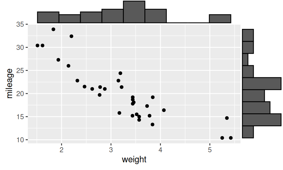
Code
dat[c("weight", "mileage")] |>
  sapply(function(x) shapiro.test(x)$p.value) |>
  round(3) |> rbind(shapiro.test = _)
weight mileage
shapiro.test 0.093 0.123Code
rho <- cor(dat$mileage, dat$weight)
TS <- rho * sqrt((n-2)/(1-rho^2))
c(cor = rho,
  TS = TS,
  q = qt(c(L = 0.025, U = 0.975), df = n-2),
  p.value = 2*pt(TS, df = n-2)
) |> round(3)
cor TS q.L q.U p.value
-0.868 -9.559 -2.042 2.042 0.000 Code
cortest.perm <- function(x, y, H1 = c("two.sided", "less", "greater"),
                          conf.level = 0.95, N = 1000) {
  # initials
  n <- length(x)
  a <- 1 - conf.level
  # calculation
  rho <- cor(x,y)
  rho.sim <- replicate(N, cor(sample(x, n, replace = FALSE),
                            sample(y, n, replace = FALSE))
                     ) # sample from H0 population
  quan <- switch(H1[1],
                 two.sided = quantile(rho.sim, probs = c(a/2, 1-a/2),
                                      names = FALSE) |> setNames(c("qL", "qU")),
                 less = c(qL = quantile(rho.sim, a, names = F), qU = 1),
                 greater = c(qL = -1, qU = quantile(rho.sim, 1-a, names = F))
  )
  pval <- switch(H1[1],
                 two.sided = 2 * min(sum(rho>rho.sim), sum(rho<rho.sim)) / N,
                 less = sum(rho.sim < rho) / N,
                 greater = sum(rho < rho.sim) /N
  )
  # output
  c(cor = rho,
    quan,
    p.value = pval
  )
}

# evaluation
cortest.perm(dat$mileage, dat$weight, H1 = "two.sided") |>
  signif(3)
cor qL qU p.value
-0.868 -0.336 0.362 0.000 Code
cor.test(~ weight + mileage, data = dat)
    Pearson's product-moment correlation

data:  weight and mileage
t = -9.559, df = 30, p-value = 1.294e-10
alternative hypothesis: true correlation is not equal to 0
95 percent confidence interval:
 -0.9338264 -0.7440872
sample estimates:
       cor
-0.8676594
All approaches reject null hypothesis, thus it is reasonable to believe that the two continuous variables are significantly (and strongly) correlated.
3.4.2 Discrete
Hypothesis about no association between two categorical variables can be tested by a well-known Pearson’s chi-squared test. First step is the construction of bivariate table of observed frequency (aka contingency/cross table) \(\{n_{ij}\}_{i,j=1}^{r,c}\). Test statistic is defined as \[ TS = \sum_{i=1}^r\sum_{j=1}^c\frac{(n_{ij}-\bar n_{ij})^2}{\bar n_{ij}} \qquad\text{with}\quad \bar n_{ij}=\frac{n_{i\boldsymbol{\cdot}}n_{\boldsymbol{\cdot}j}}{n} \] where \(\bar n_{ij}\) denotes expected frequency, \(n_{i\boldsymbol{\cdot}} = \sum_{j=1}^cn_{ij}\) is sum of all elements in row \(i\), and analogically \(n_{\boldsymbol{\cdot}j} = \sum_{i=1}^rn_{ij}\) is \(j\)-th column sum. If null hypothesis is true (RVs are independent), then test statistic asymptotically follows \(\chi^2\) distribution with \((r-1)(c-1)\) degrees of freedom.
To illustrate the matter, let us test whether type of transmission is associated with number of cylinders.
Code
# calculate
obs <- xtabs(~ transmission + cylinders, data = dat)
exp <- outer(rowSums(obs), colSums(obs)) / n
# show
obs |>
  addmargins() |>
  pander::pander(caption = "Observed frequency")
exp |>
  round(1) |>
  addmargins() |>
pander::pander(caption = "Expected frequency")| 4 | 6 | 8 | Sum | |
|---|---|---|---|---|
| automatic | 3 | 4 | 12 | 19 |
| manual | 8 | 3 | 2 | 13 |
| Sum | 11 | 7 | 14 | 32 |
| 4 | 6 | 8 | Sum | |
|---|---|---|---|---|
| automatic | 6.5 | 4.2 | 8.3 | 19 |
| manual | 4.5 | 2.8 | 5.7 | 13 |
| Sum | 11 | 7 | 14 | 32 |
Code
TS <- sum( (obs - exp)^2 / exp )

c(TS = TS,
  qU = qchisq(0.95, df = prod(dim(obs)-1)),
  p.value = 1 - pchisq(TS, df = prod(dim(obs)-1))
  ) |>
  round(3) |> rbind() |>
  pander::pander(caption = "Chi-squared distr.")
obs |>
  chisq.test(simulate.p.value = TRUE) |>
pander::pander(caption = "Simulated distr.")| TS | qU | p.value |
|---|---|---|
| 8.741 | 5.991 | 0.013 |
| Test statistic | df | P value |
|---|---|---|
| 8.741 | NA | 0.004498 * * |
Simulation of test statistic sample distribution is more appropriate when the expected cell count assumption is violated. In either case the hypothesis of independence should be rejected with 95% confidence.
Effect of each cell can be represented by residuals \(r_{ij} = (n_{ij}-\bar n_{ij}) / \sqrt{\bar n_{ij}}\), or better, by percentage they contribute to test statistic, i.e. \(r_{ij}^2/TS\).
Code
( (obs-exp) / sqrt(exp) ) |>
  round(2) |>
  pander::pander(caption = "Residuals")
( ( ( (obs-exp)^2/exp ) / TS ) * 100 ) |>
  round() |>
pander::pander(caption = "Percentual contribution to TS")| 4 | 6 | 8 | |
|---|---|---|---|
| automatic | -1.38 | -0.08 | 1.28 |
| manual | 1.67 | 0.09 | -1.55 |
| 4 | 6 | 8 | |
|---|---|---|---|
| automatic | 22 | 0 | 19 |
| manual | 32 | 0 | 27 |
3.4.3 Continuous and discrete
3.4.3.1 Binary
Association of binary and continuous RV can be checked either by the well known (independent) two-sample Student’s t-test, when assumptions (normality, no outliers) for parametric test hold, or otherwise by non-parametric alternative, the Wilcoxon rank-sum (aka Mann-Whitney U) test. The first one compares mean value of continuous RV across groups given by the binary RV, while the second one studies the shift in median (assuming similar shape and dispersion, otherwise interpretation is less straightforward).
Let \(n_1,n_2\) be sample sizes (so that \(n_1+n_2=n\)), \(\hat\mu_1,\hat\mu_2\) mean values and \(\hat\sigma_1^2,\hat\sigma_2^2\) variances in respective groups, then \[ \hat\sigma_{12}^2 = \frac{(n_1-1)\hat\sigma_1^2 + (n_2-1)\hat\sigma_2^2}{n_1+n_2-2} \] is known as pooled variance of the two samples and the test statistic of t-test defined by \[ TS = \frac{\hat\mu_1-\hat\mu_2}{\hat\sigma_{12}\sqrt{\frac1{n_1}+\frac1{n_2}}} \] follows t-distribution with degrees of freedom \(df = n_1+n_2-2\). However, if the variances are not similar, a modification known as Welch’s t-test is preferred, with \[ TS = \frac{\hat\mu_1-\hat\mu_2}{\sqrt{\frac{\hat\sigma_1^2}{n_1}+\frac{\hat\sigma_2^2}{n_2}}}\quad \text{and} \quad df = \frac{\left(\frac{\hat\sigma_1^2}{n_1}+\frac{\hat\sigma_2^2}{n_2}\right)^2}{\frac{(\hat\sigma_1^2/n_1)^2}{n_1-1} + \frac{(\hat\sigma_2^2/n_2)^2}{n_2-1}}. \] Statistical equality of two variances (\(H_0\)) can be tested by Fisher’s F-test when the test statistic \[ F = \frac{\hat\sigma_1^2}{\hat\sigma_2^2} \] under null follows Fisher-Snedecor F-distribution with \((n_1-1)\) and \((n_2-1)\) degrees of freedom.
As for the non-parametric, Mann-Whitney U test, the U statistic is given by \[ U = \sum_{i=1}^{n_1}\sum_{j=1}^{n_2}S(x_{1i}, x_{2j})\quad\text{with}\quad S(x,y)=\begin{cases}1 & \text{if} & x>y \\ 1/2 &&x=y \\ 0 && x<y \end{cases} \] where \(x_{kl}\) is \(l\)-th observation of continuous RV corresponding to \(k-th\) value of discrete RV. Under validity of null hypothesis and without ties the test statistic \(U\) asymptoticaly comes from \(N(n_1n_2/2, n_1n_2(n_1+n_2+1)/12)\). With many ties there needs to be added a correction term to the variance parameter.
Now let’s find out, whether transmission type may have effect on mileage.
Code
# EDA
ggplot(dat) + aes(x = mileage, y = transmission) +
  geom_boxplot(notch = TRUE, varwidth = TRUE)
# normality
dat |>
  dplyr::group_by(transmission) |>
  dplyr::summarize(shapiro = shapiro.test(mileage)$p.value |> round(3)) |>
  pander::pander(caption = "Normality test p-value")
# variance equality
var.test(mileage ~ transmission, data = dat) |>
  pander::pander()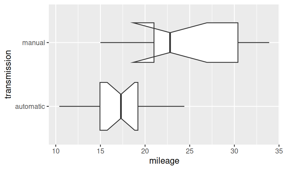
| transmission | shapiro |
|---|---|
| automatic | 0.899 |
| manual | 0.536 |
| Test statistic | num df | denom df | P value | Alternative hypothesis |
|---|---|---|---|---|
| 0.3866 | 18 | 12 | 0.06691 | two.sided |
| ratio of variances |
|---|
| 0.3866 |
Code
t.test(mileage ~ transmission, dat, var.equal = TRUE) |>
pander::pander()| Test statistic | df | P value | Alternative hypothesis |
|---|---|---|---|
| -4.106 | 30 | 0.000285 * * * | two.sided |
| mean in group automatic | mean in group manual |
|---|---|
| 17.15 | 24.39 |
Code
t.test(mileage ~ transmission, dat, var.equal = FALSE) |>
pander::pander()| Test statistic | df | P value | Alternative hypothesis |
|---|---|---|---|
| -3.767 | 18.33 | 0.001374 * * | two.sided |
| mean in group automatic | mean in group manual |
|---|---|
| 17.15 | 24.39 |
Code
wilcox.test(mileage ~ transmission, dat) |>
pander::pander()| Test statistic | P value | Alternative hypothesis |
|---|---|---|
| 42 | 0.001871 * * | two.sided |
The effect of transmission type seems to be significant, its size can be represented, e.g., by Cohen’s \(d=(\hat\mu_1-\hat\mu_2)/\hat\sigma_{12}\).
Code
rstatix::cohens_d(dat, mileage ~ transmission, var.equal = T)$effsizeCohen's d
-1.477947 According to the classification table the effect size of magnitude 1.5 is very large.
3.4.3.2 In general
Whenever the discrete RV can attain more than two values, one needs to switch from t-test to one-way analysis of variance (ANOVA) in parametric and from Mann-Whitney to Kruskal-Wallis test in non-parametric case.
Again, there are methods of ANOVA assuming similar variances in groups (samples) or, conversely, differing across groups. To test samples for homogeneity of variances the Bartlett test can be used.
We will test whether number of cylinders has significant effect upon mileage.
Code
# EDA
ggplot(dat) + aes(x = displacement, y = cylinders) +
  geom_boxplot(varwidth = TRUE)
# normality
dat |>
  dplyr::group_by(cylinders) |>
  dplyr::summarize(shapiro = shapiro.test(displacement)$p.value |> round(3)) |>
  pander::pander(caption = "Normality test p-value")
# variance equality
bartlett.test(displacement ~ cylinders, data = dat) |>
  pander::pander()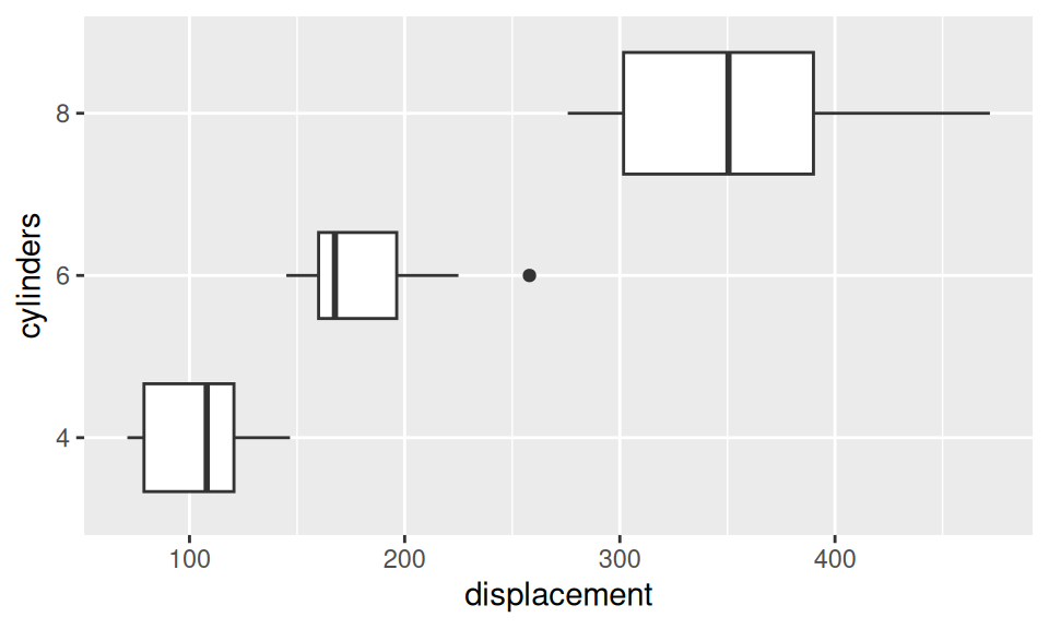
| cylinders | shapiro |
|---|---|
| 4 | 0.256 |
| 6 | 0.043 |
| 8 | 0.131 |
| Test statistic | df | P value |
|---|---|---|
| 8.166 | 2 | 0.01686 * |
Difference in location is pretty much visible from the box-whiskers plot. Normality may be violated in the group of 6-cylinder engines and variances are probably heterogeneous.
Code
oneway.test(displacement ~ cylinders, dat, var.equal = FALSE) |>
pander::pander()| Test statistic | num df | denom df | P value |
|---|---|---|---|
| 76.89 | 2 | 14.89 | 1.423e-08 * * * |
Code
kruskal.test(displacement ~ cylinders, dat) |>
pander::pander()| Test statistic | df | P value |
|---|---|---|
| 26.68 | 2 | 1.61e-06 * * * |
Both tests have clearly rejected null hypothesis about equality of distributions location in all groups.
3.4.4 Multiple comparison and post hoc tests
Rejection of the null hypothesis by the ANOVA test tells us that the means are different. But which means? All of them? Some of them? The obvious strategy is to test all possible comparisons of two means.
For inspiring explanation of multiple comparison see e.g. Navarro (2018, chapter 14.5), here we follow Dalpiaz (2018, chapter 12.4)
Let us have a data of blood coagulation (in seconds) measured on a sample of 24 animals that were randomly assigned to one of the four different diets (A,B,C,D). We first show the means for each group, then perform ANOVA test to check for evidence against the null hypothesis of equality among groups (in terms of mean) and finally perform pairwise comparison.
Code
data(coagulation, package="faraway")
ggplot(coagulation) + aes(x = coag, y = diet) + geom_boxplot()
aggregate(coag ~ diet, data = coagulation, FUN = mean) |>
  pander::pander(caption = "Group means")
oneway.test(coag ~ diet, data = coagulation, var.equal = T) |>
  pander::pander()
with(coagulation, pairwise.t.test(coag, diet, p.adj = "none")) |> pander::pander()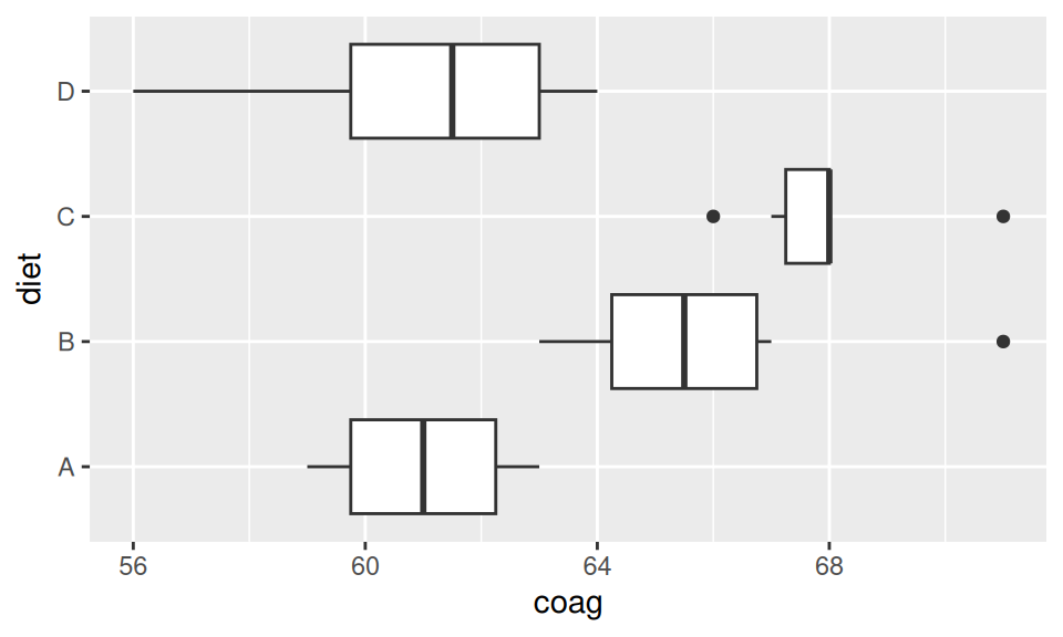
| diet | coag |
|---|---|
| A | 61 |
| B | 66 |
| C | 68 |
| D | 61 |
| Test statistic | num df | denom df | P value |
|---|---|---|---|
| 13.57 | 3 | 20 | 4.658e-05 * * * |
method: t tests with pooled SD
data.name: coag and diet
p.value:
A B C B 0.003803 NA NA C 0.0001805 0.1588 NA D 1 0.0008636 2.318e-05 p.adjust.method: none
There is strong evidence of diet type having impact on coagulation time (p-value < 0.01) so the post hoc tests are in place. It seems that differences between A-B, A-C, B-D and C-D are significant.
However, what does that note “P value adjustment method: none” in the last line mean? It is an adjustment (in this case not an adjustment) to the p-value of each test. Why would we need to adjust p-values?
The adjustment is an attempt to correct for the multiple testing problem (see also commics). Imagine that you knew ahead of time that you were going to perform large number (100) of t-tests. Suppose you wish to do this with a false positive rate of α = 0.05. If we use this significance level for each test, i.e. for 100 tests, we then expect 5 false positives. That means, with 100 tests, we’re almost guaranteed to have at least one error.
What we’d really like, is for the family-wise error rate to be 0.05. If we consider the 100 tests to be a single “experiment”, the family-wise error rate is the rate of one or more false positives in the full experiment (100 tests). Consider it an error rate for an entire procedure, instead of a single test.
With this in mind, one of the simplest adjustments we can make, is to increase the p-values for each test, depending on the number of tests. In particular a Bonferroni correction simply multiplies every p-value by the number of tests.
Code
with(coagulation, pairwise.t.test(coag, diet, p.adj = "bonferroni"))
    Pairwise comparisons using t tests with pooled SD

data:  coag and diet

  A       B       C
B 0.02282 -       -
C 0.00108 0.95266 -
D 1.00000 0.00518 0.00014

P value adjustment method: bonferroni
We see that these p-values are much higher than the unadjusted p-values, thus, we are less likely to reject each tests. As a result, the family-wise error rate is 0.05, instead of an error rate of 0.05 for each test.
To illustrate this point, we can simulate the 100 test scenario. In each test two samples (of size \(n=10\)) from the same population are compared so it is clear that H0 holds. Now suppose the 100 tests belong to one group (family) that we wish to perform within one experiment. And we wish to do it with 5% (false positive) error rate, that is \(\alpha=0.05\). If we use this significance level for each test, we then expect 5 false positives among 100 trials. That means, with 100 tests, we’re almost guaranteed to have at least one error.
What we’d really like is 5% family-wise error rate, that is \(\alpha=0.05\) for the whole experiment instead of for single test.
Code
get_p_value <- function() {
   # create data for two groups, equal mean
   y = rnorm(20, mean = 0, sd = 1)
   g = c(rep("A", 10), rep("B", 10))
   # p-value of t-test when null is true
   t.test(y ~ g, var.equal = TRUE)$p.value
}
set.seed(1337)
# family error rate if no correction applied
any(replicate(100, get_p_value()) < 0.05) |>  # Is there at least one rejection?
  replicate(n = 1000) |>
  mean()
[1] 0.994Code
# family error rate with Bonferroni correction applied
any(p.adjust(replicate(100, get_p_value()), "bonferroni") < 0.05) |>
  replicate(n = 1000) |>
  mean()
[1] 0.058Although the Bonferroni correction is the simplest adjustment out there, it’s not usually the best one to use. One method that is often used instead is the Holm correction (Holm, 1979). The idea behind the Holm correction is to pretend that we are doing the tests sequentially; starting with the smallest (raw) p-value and moving onto the largest one. The adjusted p-value is calculated as multiplication of the raw p-value and its rank, for instance in our case the smallest p-value is multiplied by 6 and the largest by 1.
Code
with(coagulation, pairwise.t.test(coag, diet)) # p.adj = "holm" is the default
    Pairwise comparisons using t tests with pooled SD

data:  coag and diet

  A       B       C
B 0.01141 -       -
C 0.00090 0.31755 -
D 1.00000 0.00345 0.00014

P value adjustment method: holm
Although it’s a little harder to calculate, the Holm correction has some very nice properties: it’s more powerful than Bonferroni (i.e., it has a lower Type II error rate), but – counterintuitive as it might seem – it has the same Type I error rate.
From the other less conservative (than the Bonferroni) approaches let us mention the so-called Tukey’s honest significant differences method useful (more sensitive) for pairwise comparisons or Scheffe’s method, which in turn is most useful (sensitive) for complex post hoc comparisons, see e.g. Hinton (2004, Chapter 13).
Code
TukeyHSD( aov(coag ~ diet, data = coagulation) ) Tukey multiple comparisons of means
95% family-wise confidence level
Fit: aov(formula = coag ~ diet, data = coagulation)
$diet
diff lwr upr p adj
B-A 5 0.7245544 9.275446 0.0183283
C-A 7 2.7245544 11.275446 0.0009577
D-A 0 -4.0560438 4.056044 1.0000000
C-B 2 -1.8240748 5.824075 0.4766005
D-B -5 -8.5770944 -1.422906 0.0044114
D-C -7 -10.5770944 -3.422906 0.00012683.5 References
- Caffo, B. 2016. Statistical Inference for Data Science.
- Dalpiaz, D. 2018. Applied Statistics with R
- Irizarry, R.A, and Love, M.I. 2016. Data Analysis for the Life Sciences with R.
- Hinton, P. 2004. Statistics Explained.
- Navarro, D. 2018. Learning Statistics with R